Transcription
accepted for publication in The Astrophysical Journal on 2012 October 9SLAC-PUB-15263Preprint typeset using LATEX style emulateapj v. 5/2/11HERSCHEL PACS AND SPIRE OBSERVATIONS OF BLAZAR PKS 1510 089:A CASE FOR TWO BLAZAR ZONESKrzysztof Nalewajko1 , Marek Sikora2 , Greg M. Madejski3 , Katrina Exter4 , Anna Szostek3,5 ,Ryszard Szczerba6 , Mark R. Kidger7 and Rosario Lorente7accepted for publication in The Astrophysical Journal on 2012 October 9ABSTRACTWe present the results of observations of blazar PKS 1510 089 with the Herschel Space Observatory PACS and SPIRE instruments, together with multiwavelength data from Fermi/LAT, Swift,SMARTS and SMA. The source was found in a quiet state, and its far-infrared spectrum is consistentwith a power-law with a spectral index of α 0.7. Our Herschel observations were preceded bytwo ‘orphan’ gamma-ray flares. The near-infrared data reveal the high-energy cut-off in the mainsynchrotron component, which cannot be associated with the main gamma-ray component in a onezone leptonic model. This is because in such a model the luminosity ratio of the External-Comptonand synchrotron components is tightly related to the frequency ratio of these components, and inthis particular case an unrealistically high energy density of the external radiation would be implied.Therefore, we consider a well-constrained two-zone blazar model to interpret the entire dataset. Inthis framework, the observed infrared emission is associated with the synchrotron component produced in the hot-dust region at the supra-pc scale, while the gamma-ray emission is associated withthe External-Compton component produced in the broad-line region at the sub-pc scale. In addition,the optical/UV emission is associated with the accretion disk thermal emission, with the accretiondisk corona likely contributing to the X-ray emission.Subject headings: galaxies: active — gamma rays: galaxies — infrared: galaxies — quasars: individual:PKS 1510 089 — quasars: jets — radiation mechanisms: non-thermal1. INTRODUCTIONOf the many classes of Active Galactic Nuclei (AGN),blazars offer the most direct insight into the extremeplasma physics of powerful relativistic jets. The spectraof blazars span the entire range of the electromagneticradiation accessible to observational techniques and areroutinely observed in the radio, millimeter, near-infrared(NIR), optical, UV, X-ray and gamma-ray bands. Evenwith this enormous observational scope, we still lack aconsistent theoretical picture of the dissipation and radiative processes responsible for this mostly non-thermaland strongly variable emission.The far-infrared (FIR) window to the Universe is rarelyaccessible owing to scarce availability of suitable observatories. Clegg et al. (1983) combined data from theKuiper Airborne Observatory at 107 µm and 240 µm,and 400 µm data from the UKIRT telescope, with otherNIR, mm and radio observations to construct the fullinfrared spectral energy distribution (SED) of blazar3C 273. Their observations can be modeled remarkably1 University of Colorado, UCB 440, Boulder, CO 80309, USA;knalew@colorado.edu2 Nicolaus Copernicus Astronomical Center, Bartycka 18, 00716 Warsaw, Poland3 Kavli Institute for Particle Astrophysics and Cosmology,SLAC National Accelerator Laboratory, Stanford University,2575 Sand Hill Road M/S 29, Menlo Park, CA 94025, USA4 Instituut voor Sterrenkunde, KU Leuven, Celestijnenlaan200 D, B-3001 Leuven, Belgium5 Astronomical Observatory, Jagiellonian University, 30-244Kraków, Poland6 Nicolaus Copernicus Astronomical Center, Rabiańska 8, 87100, Toruń, Poland7 Herschel Science Centre, ESAC, P.O. Box 78, 28691 Villanueva de la Cañada, Madrid, Spainwell with a single synchrotron component. Many blazarswere observed by the Infrared Astronomical Satellite(IRAS; e.g. Impey & Neugebauer 1988) between 12 µmand 100 µm. The interpretation of their infrared spectraas synchrotron emission was strengthened by the detection of significant variability in these sources. Haas et al.(1998) observed some blazars with the Infrared SpaceObservatory between 5 µm and 200 µm. Three of theblazars had spectra consistent with a single synchrotroncomponent, while in 3C 279 a thermal component wastentatively detected. Ogle et al. (2011) observed another prominent blazar, 3C 454.3, with the Spitzer SpaceTelescope, using all three instruments – IRS, IRAC andMIPS. They found hints of complex structure in the spectral range of MIPS (24 µm – 160 µm), which they interpreted as possible evidence for two independent synchrotron components. Another interesting result involving the Spitzer data was reported by Hayashida et al.(2012). They detected a sharp spectral break in blazar3C 279 in the MIPS spectral range, with a very hardspectral index of α 0.35 0.23 (Fν ν α ) between70 µm and 160 µm. Combined with the overall spectral shape and multiwavelength variability characteristics, this finding was also interpreted in terms of twodistinct synchrotron components.The structure of the synchrotron spectral componentin blazars is of great importance for understanding thephysical structure of the so-called “blazar zone” in relativistic AGN jets. It became clear that more detailed FIRobservations of blazars are needed. A great opportunitycame with the launch of the Herschel Space Observatory.In this work, we present photometric observations of another prominent blazar, PKS 1510 089, with two Herschel instruments – PACS and SPIRE. These results areWork supported by US Department of Energy contract DE-AC02-76SF00515 and NASA.
2Nalewajko et al.combined with the publicly available multiwavelengthdata from Fermi/LAT, Swift, SMARTS and the Submillimeter Array (SMA). PKS 1510 089 was observedpreviously in the mid-IR (MIR) band with Spitzer (IRS,IRAC and MIPS) by Malmrose et al. (2011), who lookedfor signatures of thermal emission from the dusty torusbut found the source spectrum to be consistent with apower-law. It is also a prominent gamma-ray source. Inthe spring of 2009, it showed a series of strong gammaray flares that were probed by Fermi/LAT (Abdo et al.2010b) and AGILE (D’Ammando et al. 2011). During this time, it was also detected at very-high energies( 0.1 – 1 TeV) by the H.E.S.S. observatory (Wagner &Behera 2010), as one of a handful of FSRQs known atthese energies.In Section 2, we report on our Herschel observationsand other multiwavelength data. In Section 3, we presentthe observational results, in particular multiwavelengthlight curves and quasi-simultaneous SEDs. In Section4, we present our model of the broad-band SED ofPKS 1510 089. In Section 5, we discuss how our results compare to previous studies of PKS 1510 089. Ourconclusions are given in Section 6.In this work, symbols with a numerical subscriptshould be read as a dimensionless number Xn X/(10n cgs units). We adopt a standard ΛCDM cosmology with H0 71 km s 1 Mpc 1 , Ωm 0.27 and ΩΛ 0.73, in which the luminosity distance to PKS 1510 089(z 0.36) is dL 1.91 Gpc.2. OBSERVATIONS2.1. HerschelWe observed PKS 1510 089 with the Herschel SpaceObservatory (Pilbratt et al. 2010), using the PACS(Poglitsch et al. 2010) and SPIRE (Griffin et al. 2010)instruments, in 5 epochs denoted as ‘H1’ – ‘H5’ between2011 Aug 1 (MJD 55774) and 2011 Sep 10 (MJD 55814)– see Table 1. The PACS and SPIRE observations foreach epoch took place no more than one day apart.2.1.1. Data ReductionThe PACS observations8 are mini-scan maps taken inpairs with scan and cross-scan positional angles of 70 and 110 , respectively, and with ten scan legs, each of3.5′ length and 2′′ separation. For each epoch, the PACSobservations were repeated to cover the blue red andthe green red bands. The characteristic wavelengths forthe red, green and blue bands are 160 µm, 100 µm and70 µm, respectively. Both medium and fast scan speedswere used. The SPIRE observations9 used the standardsmall-scan map method, and each observation returnedfluxes in three bands: short (PSW; 250 µm), medium(PMW; 350 µm) and long (PLW; 500 µm). The detailsare recorded in Table 1, including the date, observationID, and (for PACS) the filter and scan speed.The PACS observations were reduced using HIPE,a Herschel -specific software package (Ott 2010). Weused the Track 9 pipeline starting from Level 0, and8 The PACS Observer’s Manual is available at http://herschel.esac.esa.int/Docs/PACS/html/pacs om.html.9 The SPIRE Observer’s Manual is available at http://herschel.esac.esa.int/Docs/SPIRE/html/spire om.html.Table 1Herschel observing log for PKS 1510 089epochMJDfilterH155774.55790.55794.55806 – 55807.55813 – 55814.r br gr br gr br gr br gr br gH2H3H4H5PACSOIDsxs24997 2499825102 2510326661 2666226709 2671027007 2700827041 2704227805 2780627833 2783428361 2836228393 28394speeds 28355Note. — Individual observations have unique identifiers (OID).For each observational epoch (first column), we performed fourscanning-mode observations with PACS (s – scan, xs – cross-scan),each with a combination of two filters out of three (r – red, g –green, b – blue) and one of two scanning speeds (m – medium, f –fast); as well as one small-map observation with SPIRE.with the calibration tree v32. The pipeline tasks included crosstalk correction, non-linearity correction andsecond-level de-glitching (mapDeglitch task with thetimeordered option on). The background was removedusing the high-pass filter method, adopting filter widthsof 15, 20 and 35 readouts for blue, green and red bands,respectively; source masking radius of 25′′ for all bands;and drop size (pixfrac) of 1. The map pixel sizes are1.1′′ , 1.4′′ and 2.1′′ for the blue, green and red bands,respectively.The SPIRE observations were also reduced using theHIPE, with the Track 9 pipeline starting from Level0.5, and with the calibration version spire cal 1. Toremove the background, we used the destriping taskwith standard parameter settings. The maps were madewith pixel sizes of of 6′′ , 10′′ and 14′′ for the PSW, PMWand PLW bands, respectively. Background sources werefitted and removed with the source extractor routine (removing only those that appeared at all epochs). TheSPIRE maps were converted to the units of Jy/pix, tomatch the units of the PACS maps, using the recommended beam-to-pixel size conversion factors.2.1.2. PhotometryAll maps were measured for photometric fluxes using the aperture photometry with recommended aperturesizes for the source and the sky, and published aperturecorrections10. For SPIRE, we obtained two additionalflux measurements by fitting the source on the map (astandard HIPE task) and along the timeline11. Thefinal adopted flux value is the mean of the three measurements, with the differences between results for eachepoch never exceeding 0.01 Jy ( 2%). The calibrationuncertainties are reported to be 5% for PACS and 7%for SPIRE. No color corrections were applied to the measured fluxes, the SPIRE and PACS calibration assume asource spectral index of α 1 (Fν ν α ).10 “PACS instrument and calibration” – /PacsCalibrationWeb;“SPIRE instrument and calibration” – /SpireCalibrationWeb.11We used a script provided by the SPIRE team:bendoSourceFit v9.py.
Herschel observations of PKS 1510 0893Table 2Photometric results of Herschel PACS and SPIRE observations of PKS 1510 089blue (70µ)H1 (MJD 55774)0.52 0.010.46 0.01H2 (MJD 55790)H3 (MJD 55794)0.48 0.01H4 (MJD 55806 – 55807) 0.39 0.01H5 (MJD 55813 – 55814) 0.38 0.01Note. — The fluxes are given in units of Jy.PACSgreen (100µm)0.36 0.020.33 0.020.35 0.020.28 0.020.31 0.02red (160µm)0.29 0.020.22 0.020.25 0.020.20 0.020.22 0.02In all six bands, we checked whether PKS 1510 089 isa point source. We computed the radial flux profiles bymeasuring the flux in apertures of increasing radius, andcompared them to the flux profiles produced from thePSF maps for each instrument (PACS: from FITS filesprovided on the instrument public page; SPIRE: from acalibration file). In all cases, the blazar was compatiblewith a point source.For the PACS maps, we had a mixture of the fast andmedium scan speeds: observations in the green band weretaken with the fast scan speeds only, and those in the blueand red bands were taken with either of the two scanspeeds. The available aperture corrections have beenproduced only for the medium (and slow) scan speeds,hence for the fast scan speeds there is an additional uncertainty of a few percent in the flux measurement (basedon a comparison of their PSFs: PACS team communication). In addition, the signal-to-noise ratio is slightlyworse on the fast scan speed maps. Therefore, we usedonly the medium scan speed map fluxes for the red andblue bands, and the average of the fast scan speed mapfluxes for the green band. To check on the difference inphotometry between scan speeds, we compared the results for fast and medium scan speed maps in the redand green: the difference is not greater than 0.02 Jy forboth bands. This value is similar to the typical flux measurement errors (see Table 2).For all maps we measure the scatter in the backgroundas the standard deviation between about 8 aperturesplaced in background regions, which currently is the bestmethod of estimating the flux measurement uncertainty.Since the background is devoid of any obvious traces ofthe interstellar medium, the observing mode is the samefor all the epochs, and the data are reduced in the sameway, we report only one average flux error for each of the6 bands covered by PACS and SPIRE. The final resultsof the PACS and SPIRE photometry of PKS 1510 089are reported in Table 2.2.2. Fermi/LATThe Fermi/LAT telescope (Atwood et al. 2009) formost of 2011 operated in the scanning mode, observing the entire sky frequently and fairly uniformly. Weused the standard analysis software package ScienceTools v9r27p1, with the instrument response functions P7SOURCE V6 (Fermi-LAT Collaboration 2012),the Galactic diffuse emission model gal 2yearp7v6 v0and the isotropic background model iso p7v6source.Events of the SOURCE class were extracted from the regionof interest (ROI) of 10 radius centered on the positionof PKS 1510 089 (α 228.2 , δ 9.1 ). The background model included 17 sources from the Fermi/LATPSW (250µm)0.67 0.020.61 0.020.64 0.020.55 0.020.57 0.02SPIREPMW (350µm)0.83 0.020.79 0.020.84 0.020.72 0.020.74 0.02PLW (500µm)0.99 0.010.96 0.011.02 0.010.92 0.010.93 0.01Second Source Catalog (Nolan et al. 2012) within 15 from PKS 1510 089; their spectral models are powerlaws with the photon index fixed to the catalog values, and for sources outside the ROI the normalizations were also fixed. In addition, our source model included TXS 1530 131, located 6 from PKS 1510 089,which was in a flaring state (Gasparrini & Cutini 2011).The free parameters of the source model are: the normalizations of all point sources within ROI, as well asof the diffuse components, and the photon indices ofPKS 1510 089 and TXS 1530 131. The source fluxwas calculated with the unbinned maximum likelihoodmethod, following standard recommendations12 (zenithangle 100 and the gtmktime filter (DATA QUAL 1)&& (LAT CONFIG 1) && ABS(ROCK ANGLE) 52). Measurements with the test statistic TS 10 (Mattox et al.1996) and with the predicted number of gamma raysNpred 3 are presented in figures as data points. Forthe SEDs, we also plot 2-σ upper limits calculated witha method described in Section 4.4 of Abdo et al. (2010c).To calculate the medium-term light curve, we selectedevents registered between MJD 55740 and MJD 55830of reconstructed energy between Emin 200 MeV andEmax 300 GeV. The spectrum of PKS 1510 089 wasmodeled with a power-law with a free photon index. Thelight curve is presented with overlapping 3-day bins witha 1-day time step. The νFν values are calculated from thefitted power-law model at photon energies of 200 MeVand 2 GeV.To calculate the long-term light curve, we selectedevents between MJD 54700 and MJD 55840, and modeled them in 6-day bins. We used the same energy rangeas before, and the νFν values correspond to the photonenergy of 2 GeV.To calculate the SEDs, we selected events registeredover 3-day time intervals (MJD 55789 – 55792 for the‘H2’ state, MJD 55766 – 55769 for the ‘F2’ state; seebelow) in overlapping energy bins of equal logarithmicwidth and uniform logarithmic spacing:Emin EmaxEmin (i k)/N E Emin EmaxEmin i/N(1)with Emin 100 MeV, Emax 100 GeV, k 3, N 18and i {k, ., N }. Within each bin, the spectrum ofPKS 1510 089 was modeled with a power-law with afixed photon index determined from power-law fits in thebroad energy range 200 MeV E 300 GeV: ΓH2 2.44 and ΓF2 s/documentation/Cicerone/
4Nalewajko et al.Table 3Results of Swift/XRT observations of PKS 1510 089Obs 140Countsbkg40.3–10 keV Flux10 12 erg cm 2 s 17.42 1.58 1.003ΓX1.68 0.17 0.17Norm10 3 keV 1 cm 2 s 11.05 0.14 0.13Reducedχ20.491.48 0.33 0.310.86 0.17 0.162.261.40 0.09 0.091.53 0.08 0.080.90 0.07 0.071.01 0.06 855749.323853.7253567.34 2.82 1.598.38 1.04 0.888.16 0.82 028413–10.00 1.69 1.40–1.52 0.13 0.13–1.22 0.10 0.113117308155762.481667.3522459.20 1.80 1.481.39 0.14 0.130.98 0.10 0.100.813117308255766.681995.813501610.18 1.69 1.201.52 0.11 0.101.23 0.09 0.091.733117308355768.472166.3137099.68 1.22 1.011.60 0.10 0.101.27 0.09 0.090.981.54 0.11 0.111.39 0.11 0.111.58 0.11 0.111.32 0.11 0.110.801.05 0.10 0.100.861.30 0.11 655774.192023.39330510.61 1.42 1.199.99 1.45 1.2610.04 1.50 020205–7.31 1.12 0.99–1.63 0.14 0.14–0.99 0.10 0.10–0.473117308955782.581664.85283410.42 1.26 1.171.65 0.12 0.121.43 0.13 0.130.7012.88 1.80 1.4111.79 1.54 1.349.93 1.41 1.2110.85 1.63 1.2212.38 3.42 2.4412.61 1.64 1.579.88 1.68 1.321.46 0.10 0.101.30 0.09 0.091.29 0.10 0.101.39 0.11 0.111.31 0.17 0.171.27 0.10 0.101.25 0.11 0.111.47 0.12 0.121.12 0.08 0.080.93 0.08 0.081.14 0.10 0.101.19 0.14 0.141.17 0.10 0.100.89 0.08 900.971.031.280.981.18Note. — The spectrum was fitted in the 0.3 – 10 keV band with a model wabs*powerlaw, the hydrogen column density NH was fixedat 7.9 1020 cm 2 , and the free photon index ΓX . The reported flux values correspond to the de-absorbed spectrum. Errors on thenormalization parameter and ΓX are 1σ. Flux errors correspond to 90% confidence interval using xspec script fluxerror.tcl. Backgroundcounts are scaled to the size of the source region using backscal keyword. Observations with less than 75 counts were not fitted.Table 4Results of Swift/UVOT photometry for PKS 1510 089Obs 55793.6655796.0655799.61V4.65 0.385.03 0.446.24 0.496.85 0.26–5.15 0.326.67 0.397.71 0.386.56 0.346.39 0.355.28 0.347.58 0.37–5.33 0.385.91 0.407.36 0.628.86 0.375.95 0.326.75 0.353.78 0.405.43 0.354.57 0.33B6.69 0.307.63 0.367.80 0.238.54 0.20–7.22 0.267.88 0.329.05 0.288.13 0.278.07 0.276.99 0.278.92 0.296.83 0.386.84 0.307.83 0.319.49 0.2810.79 0.286.89 0.248.34 0.276.88 0.336.77 0.306.19 0.26U6.99 0.308.32 0.368.49 0.259.24 0.238.95 0.597.72 0.278.38 0.319.55 0.308.86 0.288.88 0.297.78 0.289.02 0.298.10 0.387.11 0.288.26 0.3110.31 0.3011.49 0.317.86 0.258.90 0.287.72 0.327.77 0.287.37 0.26W16.01 0.327.21 0.397.38 0.297.83 0.306.83 0.336.65 0.307.66 0.357.88 0.347.70 0.337.97 0.346.44 0.307.81 0.346.61 0.346.19 0.317.11 0.348.94 0.3710.44 0.416.96 0.307.55 0.326.96 0.366.76 0.316.07 0.28M27.92 0.379.77 0.4510.12 0.1810.63 0.25–8.72 0.3410.15 0.3710.75 0.358.90 0.4310.41 0.339.66 0.3410.04 0.34–9.24 0.329.84 0.3712.30 0.5712.31 0.359.47 0.2910.73 0.338.80 0.549.08 0.338.85 0.33W26.71 0.279.47 0.379.65 0.2810.09 0.27–8.38 0.279.50 0.319.39 0.309.64 0.298.98 0.298.76 0.299.25 0.2911.67 1.368.54 0.309.44 0.3211.27 0.3311.35 0.339.41 0.2810.22 0.319.07 0.338.74 0.288.41 0.27Note. — We report flux densities νFν corrected for extinction, in units of 10 12 erg s 1 cm 2 . Quoted errors are a sum of 1σ statisticaland a systematic error added in quadrature. Systematic errors are of the order of 5%.
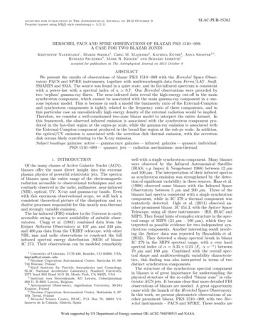
Herschel observations of PKS 1510 0892.3. Swift2.3.1. XRT Data AnalysisWe analyzed the Swift /XRT data following the recommendations given in the “Data Reduction Guide v1.2”.We used the ftools software package v6.11, the Swiftcalibration files from November 2011, and the xspec program v12.7.0. We started from Level 1 event files, andreduced the data using the xrtpipeline script with default screening and filtering criteria. With xrtpipeline,we created the exposure maps and used them to correctthe arf files for dead columns. We extracted the sourceand the background spectra, using the xselect programv2.4b, from a circular region centered on the source andwith a radius of 47′′ . The background came from anannulus centered on the source and with the inner andouter radii of 80′′ and 135′′ , respectively. To obtain thespectral parameters, we fitted observations which havemore than 75 source counts with an absorbed power-lawmodel with hydrogen column density fixed at its Galactic value of 7.9 1020 cm 2 (Kataoka et al. 2008), andwith a free photon index. To calculate the flux errors,we used a script fluxerror.tcl provided by the xspecteam13 . The results are given in Table 3.2.3.2. UVOT Data analysisTo analyze the UVOT data in the image mode, we followed the recommendations from the “UVOT SoftwareGuide v2.2”, and started from the Level 1 raw data. Weconstructed a bad pixel map for each exposure to remove the bad pixels from further analysis. We reduceda modulo8 fixed-pattern noise from the images and thepixel-to-pixel fluctuations in the images due to detectorsensitivity variations. Then, we converted the imagesfrom a raw coordinate system to tangential projectionon the sky. Before adding the images, we applied anaspect-ratio correction to each exposure to obtain thecorrect sky coordinates of the UVOT sources and to ensure that individual exposures were added without offsets. Finally, we added all image exposures for a specificfilter in a given observation. To extract the source magnitude and counts, we used the uvotsource task. Weused an aperture of 5′′ for all filters, which matches theaperture used to calibrate the UVOT photometry, andtherefore it does not require aperture corrections. Thebackground is estimated from an annulus with radii of15′′ and 25′′ centered on the source. The results are presented in Table 4.To convert the observed magnitudes mλ to flux densities νFν , we introduce an effective zero point Zλ , suchthat νFν [erg s 1 cm 2 ] 10(Zλ mλ Aλ )/2.5 , where Aλ isthe extinction. For Swift /UVOT, we took(UVOT)Zλ(P08) Zλ(P08) 2.5 log(λeff[erg s 1 cm 2 Å 1 ]) ,(P08)(P08)(P08)[Å] CF(2)(P08)where Zλ, λeffand CFare parameters takenfrom Tables 6, 8 and 10 in Poole et al. (2008), respec(P08)tively. We adopt λeff as the effective wavelength for theUVOT filters. For the extinction correction in the direction to PKS 1510 089, we adopted a standard GalacticTable 5Effective wavelengths, extinctions and effective zero points for theSMARTS (K — B) and Swift/UVOT (U — W2) xanadu/xspec/fluxerror.htmlλeff � 40extinction model by Cardelli et al. (1989) with parameters E(B V ) 0.101 and RV 3.1. In Table 5, wereport the effective wavelengths, extinctions and effective zero points for UVOT filters U, W1, M2 and W2.The effective zero points for filters V and B are consistent with the Cousins-Glass-Johnson photometric systemdiscussed in Section 2.4.2.4. SMARTS and SMAWe used public optical and NIR data (B, V, R, J andK filters) from the Yale University SMARTS project14 .A part of the data for PKS 1510 089 was presented inBonning et al. (2012). The magnitudes mλ were converted into flux densities using the effective zero pointsintroduced in Section 2.3.2, here calculated as(SMARTS)Zλ 2.5 log(νeff [Hz] fν(B98)[erg s 1 cm 2 Hz 1 ]) ,(B98)c/λeff ,(B98)λeff(3)(B98)fνwhere νeff andandare parameters of the Cousins-Glass-Johnson photometric systemtaken from Table A2 in Bessell et al. (1998). The effective wavelengths and zero points for each SMARTS filterare reported in Table 5.We obtained the SMA data for PKS 1510 089 at1.3 mm wavelength from the SMA Callibrator List15(Gurwell et al. 2007). We use these data only to verify that they lie on the power-law extrapolation of theHerschel PACS and SPIRE SED.3. RESULTS3.1. Herschel PACS and SPIREFigure 1 shows the light curves of PKS 1510 089 calculated for each filter of the PACS and SPIRE instruments. The source was not significantly variable overweekly time scales across the entire spectral range. Theslight variations observed at different wavelengths appearto be correlated.Figure 2 shows the FIR spectral energy distributions(SEDs) of PKS 1510 089 in 5 epochs; for each epochobservations in all six bands were performed within oneday. These SEDs are generally consistent with powerlaws. The parameters of the spectral fits for each observational epoch are reported in Table 6. A slight harderwhen-brighter trend is apparent, although the range ofparameter values is rather t/http://sma1.sma.hawaii.edu/callist/callist.html
6Nalewajko et al.500 µm350 µm250 µm160 µm100 µm70 µm1F [Jy]0.80.60.40.205577055775557805578555790 55795MJD55800558055581055815Figure 1. Herschel PACS (filled symbols) and SPIRE (emptysymbols) light curves of PKS 1510 089.λobs [µm]50010060(νFν)obs [erg s-1 cm-2]2e-11MJD 55774-5MJD 55790-1MJD 55794-5MJD 55806-8MJD 55813-51e-115e-125e 111e 125e 12νobs [Hz]Figure 2. Herschel PACS and SPIRE quasi-simultaneous spectral energy distributions of PKS 1510 089.Table 6Spectral fits to the Herschel PACS and SPIRE dataepochαlog(νFν [erg s 1 cm 2 ]) at 1012 HzH10.64 0.02 11.130 0.007H20.74 0.04 11.158 0.019H30.71 0.02 11.135 0.007H40.766 0.012 11.201 0.004H50.75 0.04 11.192 0.014Note. — The model is a power-law function in the form Fν ν α .3.2. Multiwavelength dataTo provide a context for the results obtained withHerschel, we analyze quasi-simultaneous multiwavelength data for PKS 1510 089: gamma-ray data fromFermi/LAT, optical/UV and X-ray data from Swift, optical/NIR data from SMARTS, and millimeter data fromSMA. In Figure 3, we present multiwavelength lightcurves calculated over a period of 3 months encompassing our Herschel campaign. The simultaneous multiwavelength coverage varies between different Herschelpointings. The Herschel observations span a period ofrelatively low activity following two prominent gammaray flares – ‘F1’ (MJD 55745; D’Ammando & Gasparrini 2011) and ‘F2’ (MJD 55767).16 The Fermi/LATdata indicate a modest spectral variability across thegamma-ray band. The F2 gamma-ray flare has a possible optical/NIR counterpart seen in the SMARTS data16Two more prominent gamma-ray flares were observed inPKS 1510 089 in Oct–Nov 2011 (Orienti et al., submitted).(see also Hauser et al. 2011). The discrete correlationfunction (Edelson & Krolik 1988) calculated between theFermi/LAT data at 2 GeV and the SMARTS data inthe V band (Figure 4) indicates that the optical fluxis delayed with respect to the gamma-ray flux by 1 2days. However, such correlation is not confirmed by theSwift /UVOT data, the brighter F1 gamma-ray flare doesnot have a similar optical counterpart, and the amplitudeof optical variability is one order of magnitude smallerthan the amplitude of the gamma-ray flare. Thus, thesetwo gamma-ray flares can be practically called ‘orphan’flares. Of the NIR/optical/UV bands, the most prominent activity is seen in the K band.We extracted the broad-band spectral energy distributions (SEDs) of PKS 1510 089 for two epochs. Thesecond Herschel pointing (H2) is chosen among otherHerschel pointings for the best overall multiwavelengthcoverage and the highest simultaneous gamma-ray flux.The second gamma-ray flare (F2) has a better multiwavelength coverage than the first gamma-ray flare. Thesetwo SEDs are shown in Figure 5. We find a very goodagreement in the NIR/optical/UV and X-ray bands between these two epochs. There is a prominent difference in the gamma-ray band, not only in the integratedluminosity, but also in the spectral shape. In the lowgamma-ray state (H2), the gamma-ray spectrum is muchsofter and can be reasonably approximated with a singlepower law. In the high gamma-ray state (F2), a possible double structure is seen, with peaks at 250 MeVand 1.5 GeV, and a dip at 700 MeV.17 The spectrum in the F2 state is significantly harder, at least upto 3 GeV. Because of such a hard spectrum, theintegrated luminosity calculated by fitting a power-la
- see Table 1. The PACS and SPIRE observations for each epoch took place no more than one day apart. 2.1.1. DataReduction The PACS observations8 are mini-scan maps taken in pairs with scan and cross-scan positional angles of 70 and 110 , respectively, and with ten scan legs, each of 3.5′ length and 2′′ separation. For each epoch, the PACS