Transcription
Learning to Track at 100 FPS with DeepRegression NetworksDavid Held, Sebastian Thrun, Silvio SavareseDepartment of Computer ScienceStanford bstract. Machine learning techniques are often used in computer vision due to their ability to leverage large amounts of training data toimprove performance. Unfortunately, most generic object trackers arestill trained from scratch online and do not benefit from the large number of videos that are readily available for offline training. We proposea method for offline training of neural networks that can track novelobjects at test-time at 100 fps. Our tracker is significantly faster thanprevious methods that use neural networks for tracking, which are typically very slow to run and not practical for real-time applications. Ourtracker uses a simple feed-forward network with no online training required. The tracker learns a generic relationship between object motionand appearance and can be used to track novel objects that do not appearin the training set. We test our network on a standard tracking benchmark to demonstrate our tracker’s state-of-the-art performance. Further,our performance improves as we add more videos to our offline trainingset. To the best of our knowledge, our tracker1 is the first neural-networktracker that learns to track generic objects at 100 fps.Keywords: Tracking, deep learning, neural networks, machine learning1IntroductionGiven some object of interest marked in one frame of a video, the goal of “singletarget tracking” is to locate this object in subsequent video frames, despite objectmotion, changes in viewpoint, lighting changes, or other variations. Single-targettracking is an important component of many systems. For person-following applications, a robot must track a person as they move through their environment.For autonomous driving, a robot must track dynamic obstacles in order to estimate where they are moving and predict how they will move in the future.Generic object trackers (trackers that are not specialized for specific classesof objects) are traditionally trained entirely from scratch online (i.e. during testtime) [15, 3, 36, 19], with no offline training being performed. Such trackers sufferin performance because they cannot take advantage of the large number of videosthat are readily available to improve their performance. Offline training videos1Our tracker is available at http://davheld.github.io/GOTURN/GOTURN.html
2Held, Thrun, SavareseTraining:Test:Training videosand imagesNeuralNetworkPrevious frameNeuralNetworkFrozen weightsCurrent frametracking outputCurrent frameNetwork learns generic object trackingNetwork tracks novel objects(no finetuning)Fig. 1. Using a collection of videos and images with bounding box labels (but noclass information), we train a neural network to track generic objects. At test time, thenetwork is able to track novel objects without any fine-tuning. By avoiding fine-tuning,our network is able to track at 100 fpscan be used to teach the tracker to handle rotations, changes in viewpoint,lighting changes, and other complex challenges.In many other areas of computer vision, such as image classification, objectdetection, segmentation, or activity recognition, machine learning has allowedvision algorithms to train from offline data and learn about the world [5, 23, 13,25, 9, 28]. In each of these cases, the performance of the algorithm improves as ititerates through the training set of images. Such models benefit from the abilityof neural networks to learn complex functions from large amounts of data.In this work, we show that it is possible to learn to track generic objects inreal-time by watching videos offline of objects moving in the world. To achievethis goal, we introduce GOTURN, Generic Object Tracking Using RegressionNetworks. We train a neural network for tracking in an entirely offline manner.At test time, when tracking novel objects, the network weights are frozen, and noonline fine-tuning required (as shown in Figure 1). Through the offline trainingprocedure, the tracker learns to track novel objects in a fast, robust, and accuratemanner.Although some initial work has been done in using neural networks for tracking, these efforts have produced neural-network trackers that are too slow forpractical use. In contrast, our tracker is able to track objects at 100 fps, making it, to the best of our knowledge, the fastest neural-network tracker to-date.Our real-time speed is due to two factors. First, most previous neural networktrackers are trained online [26, 27, 34, 37, 35, 30, 39, 7, 24]; however, training neural networks is a slow process, leading to slow tracking. In contrast, our tracker istrained offline to learn a generic relationship between appearance and motion, sono online training is required. Second, most trackers take a classification-basedapproach, classifying many image patches to find the target object [26, 27, 37, 30,39, 24, 33]. In contrast, our tracker uses a regression-based approach, requiringjust a single feed-forward pass through the network to regresses directly to thelocation of the target object. The combination of offline training and one-pass
Learning to Track3regression leads to a significant speed-up compared to previous approaches andallows us to track objects at real-time speeds.GOTURN is the first generic object neural-network tracker that is able torun at 100 fps. We use a standard tracking benchmark to demonstrate that ourtracker outperforms state-of-the-art trackers. Our tracker trains from a set of labeled training videos and images, but we do not require any class-level labelingor information about the types of objects being tracked. GOTURN establishesa new framework for tracking in which the relationship between appearance andmotion is learned offline in a generic manner. Our code and additional experiments can be found at ed WorkOnline training for tracking. Trackers for generic object tracking are typicallytrained entirely online, starting from the first frame of a video [15, 3, 36, 19]. Atypical tracker will sample patches near the target object, which are considered as“foreground” [3]. Some patches farther from the target object are also sampled,and these are considered as “background.” These patches are then used to traina foreground-background classifier, and this classifier is used to score patchesfrom the next frame to estimate the new location of the target object [36, 19].Unfortunately, since these trackers are trained entirely online, they cannot takeadvantage of the large amount of videos that are readily available for offlinetraining that can potentially be used to improve their performance.Some researchers have also attempted to use neural networks for trackingwithin the traditional online training framework [26, 27, 34, 37, 35, 30, 39, 7, 24,16], showing state-of-the-art results [30, 7, 21]. Unfortunately, neural networksare very slow to train, and if online training is required, then the resultingtracker will be very slow at test time. Such trackers range from 0.8 fps [26]to 15 fps [37], with the top performing neural-network trackers running at 1fps on a GPU [30, 7, 21]. Hence, these trackers are not usable for most practicalapplications. Because our tracker is trained offline in a generic manner, no onlinetraining of our tracker is required, enabling us to track at 100 fps.Model-based trackers. A separate class of trackers are the model-basedtrackers which are designed to track a specific class of objects [12, 1, 11]. Forexample, if one is only interested in tracking pedestrians, then one can train apedestrian detector. During test-time, these detections can be linked togetherusing temporal information. These trackers are trained offline, but they are limited because they can only track a specific class of objects. Our tracker is trainedoffline in a generic fashion and can be used to track novel objects at test time.Other neural network tracking frameworks. A related area of researchis patch matching [14, 38], which was recently used for tracking in [33], runningat 4 fps. In such an approach, many candidate patches are passed through thenetwork, and the patch with the highest matching score is selected as the trackingoutput. In contrast, our network only passes two images through the network,and the network regresses directly to the bounding box location of the target
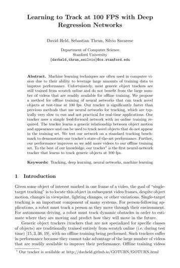
4Held, Thrun, SavareseCurrent frameSearch RegionConv LayersCropFully-ConnectedLayersCropPrevious frameWhat to trackPredicted loca3onof targetwithin search regionConv LayersFig. 2. Our network architecture for tracking. We input to the network a search regionfrom the current frame and a target from the previous frame. The network learns tocompare these crops to find the target object in the current imageobject. By avoiding the need to score many candidate patches, we are able totrack objects at 100 fps.Prior attempts have been made to use neural networks for tracking in various other ways [18], including visual attention models [4, 29]. However, theseapproaches are not competitive with other state-of-the-art trackers when evaluated on difficult tracker datasets.33.1MethodMethod OverviewAt a high level, we feed frames of a video into a neural network, and the networksuccessively outputs the location of the tracked object in each frame. We trainthe tracker entirely offline with video sequences and images. Through our offlinetraining procedure, our tracker learns a generic relationship between appearanceand motion that can be used to track novel objects at test time with no onlinetraining required.3.2Input / output formatWhat to track. In case there are multiple objects in the video, the networkmust receive some information about which object in the video is being tracked.To achieve this, we input an image of the target object into the network. Wecrop and scale the previous frame to be centered on the target object, as shownin Figure 2. This input allows our network to track novel objects that it has notseen before; the network will track whatever object is being input in this crop.We pad this crop to allow the network to receive some contextual informationabout the surroundings of the target object.In more detail, suppose that in frame t 1, our tracker previously predictedthat the target was located in a bounding box centered at c (cx , cy ) with awidth of w and a height of h. At time t, we take a crop of frame t 1 centered
Learning to Track5at (cx , cy ) with a width and height of k1 w and k1 h, respectively. This crop tellsthe network which object is being tracked. The value of k1 determines how muchcontext the network will receive about the target object from the previous frame.Where to look. To find the target object in the current frame, the trackershould know where the object was previously located. Since objects tend tomove smoothly through space, the previous location of the object will providea good guess of where the network should expect to currently find the object.We achieve this by choosing a search region in our current frame based on theobject’s previous location. We crop the current frame using the search regionand input this crop into our network, as shown in Figure 2. The goal of thenetwork is then to regress to the location of the target object within the searchregion.In more detail, the crop of the current frame t is centered at c0 (c0x , c0y ),where c0 is the expected mean location of the target object. We set c0 c, whichis equivalent to a constant position motion model, although more sophisticatedmotion models can be used as well. The crop of the current frame has a widthand height of k2 w and k2 h, respectively, where w and h are the width and heightof the predicted bounding box in the previous frame, and k2 defines our searchradius for the target object. In practice, we use k1 k2 2.As long as the target object does not become occluded and is not moving tooquickly, the target will be located within this region. For fast-moving objects, thesize of the search region could be increased, at a cost of increasing the complexityof the network. Alternatively, to handle long-term occlusions or large movements,our tracker can be combined with another approach such as an online-trainedobject detector, as in the TLD framework [19], or a visual attention model [4,29, 2]; we leave this for future work.Network output. The network outputs the coordinates of the object in thecurrent frame, relative to the search region. The network’s output consists of thecoordinates of the top left and bottom right corners of the bounding box.3.3Network architectureFor single-target tracking, we define a novel image-comparison tracking architecture, shown in Figure 2 (note that related “two-frame” architectures havealso been used for other tasks [20, 10]). In this model, we input the target objectas well as the search region each into a sequence of convolutional layers. Theoutput of these convolutional layers is a set of features that capture a high-levelrepresentation of the image.The outputs of these convolutional layers are then fed through a number offully connected layers. The role of the fully connected layers is to compare thefeatures from the target object to the features in the current frame to find wherethe target object has moved. Between these frames, the object may have undergone a translation, rotation, lighting change, occlusion, or deformation. Thefunction learned by the fully connected layers is thus a complex feature comparison which is learned through many examples to be robust to these variousfactors while outputting the relative motion of the tracked object.
6Held, Thrun, SavareseIn more detail, the convolutional layers in our model are taken from the firstfive convolutional layers of the CaffeNet architecture [17, 23]. We concatenate theoutput of these convolutional layers (i.e. the pool5 features) into a single vector.This vector is input to 3 fully connected layers, each with 4096 nodes. Finally, weconnect the last fully connected layer to an output layer that contains 4 nodeswhich represent the output bounding box. We scale the output by a factor of 10,chosen using our validation set (as with all of our hyperparameters). Networkhyperparameters are taken from the defaults for CaffeNet, and between eachfully-connected layer we use dropout and ReLU non-linearities as in CaffeNet.Our neural network is implemented using Caffe [17].3.4TrackingDuring test time, we initialize the tracker with a ground-truth bounding boxfrom the first frame, as is standard practice for single-target tracking. At eachsubsequent frame t, we input crops from frame t 1 and frame t into the network(as described in Section 3.2) to predict where the object is located in frame t. Wecontinue to re-crop and feed pairs of frames into our network for the remainderof the video, and our network will track the movement of the target objectthroughout the entire video sequence.4TrainingWe train our network with a combination of videos and still images. The trainingprocedure is described below. In both cases, we train the network with an L1loss between the predicted bounding box and the ground-truth bounding box.4.1Training from Videos and ImagesOur training set consists of a collection of videos in which a subset of framesin each video are labeled with the location of some object. For each successivepair of frames in the training set, we crop the frames as described in Section 3.2.During training time, we feed this pair of frames into the network and attemptto predict how the object has moved from the first frame to the second frame(shown in Figure 3). We also augment these training examples using our motionmodel, as described in Section 4.2.Our training procedure can also take advantage of a set of still images that areeach labeled with the location of an object. This training set of images teachesour network to track a more diverse set of objects and prevents overfitting tothe objects in our training videos. To train our tracker from an image, we takerandom crops of the image according to our motion model (see Section 4.2). Between these two crops, the target object has undergone an apparent translationand scale change, as shown in Figure 4. We treat these crops as if they were takenfrom different frames of a video. Although the “motions” in these crops are lessvaried than the types of motions found in our training videos, these images arestill useful to train our network to track a variety of different objects.
Learning to nding)box)Fig. 3. Examples of training videos. The goal of the network is to predict the locationof the target object shown in the center of the video frame in the top row, after beingshifted as in the bottom row. The ground-truth bounding box is marked in round5truth&bounding&box&Fig. 4. Examples of training images. The goal of the network is to predict the locationof the target object shown in the center of the image crop in the top row, after beingshifted as in the bottom row. The ground-truth bounding box is marked in green4.2Learning Motion SmoothnessObjects in the real-world tend to move smoothly through space. Given an ambiguous image in which the location of the target object is uncertain, a trackershould predict that the target object is located near to the location where it waspreviously observed. This is especially important in videos that contain multiplenearly-identical objects, such as multiple fruit of the same type. Thus we wishto teach our network that, all else being equal, small motions are preferred tolarge motions.To concretize the idea of motion smoothness, we model the center of thebounding box in the current frame (c0x , c0y ) relative to the center of the boundingbox in the previous frame (cx , cy ) asc0x cx w · x(1)c0y cy h · y(2)where w and h are the width and height, respectively, of the bounding box ofthe previous frame. The terms x and y are random variables that capturethe change in position of the bounding box relative to its size. In our trainingset, we find that objects change their position such that x and y can eachbe modeled with a Laplace distribution with a mean of 0 (see Supplementary
8Held, Thrun, SavareseMaterial for details). Such a distribution places a higher probability on smallermotions than larger motions.Similarly, we model size changes byw 0 w · γw0h h · γh(3)(4)where w0 and h0 are the current width and height of the bounding box and wand h are the previous width and height of the bounding box. The terms γw andγh are random variables that capture the size change of the bounding box. Wefind in our training set that γw and γh are modeled by a Laplace distributionwith a mean of 1. Such a distribution gives a higher probability on keeping thebounding box size near the same as the size from the previous frame.To teach our network to prefer small motions to large motions, we augment our training set with random crops drawn from the Laplace distributionsdescribed above (see Figures 3 and 4 for examples). Because these training examples are sampled from a Laplace distribution, small motions will be sampledmore than large motions, and thus our network will learn to prefer small motionsto large motions, all else being equal. We will show that this Laplace croppingprocedure improves the performance of our tracker compared to the standarduniform cropping procedure used in classification tasks [23].The scale parameters for the Laplace distributions are chosen via crossvalidation to be bx 1/5 (for the motion of the bounding box center) andbs 1/15 (for the change in bounding box size). We constrain the random cropsuch that it must contain at least half of the target object in each dimension. Wealso limit the size changes such that γw , γh (0.6, 1.4), to avoid overly stretchingor shrinking the bounding box in a way that would be difficult for the networkto learn.4.3Training procedureTo train our network, each training example is alternately taken from a video orfrom an image. When we use a video training example, we randomly choose avideo, and we randomly choose a pair of successive frames in this video. We thencrop the video according to the procedure described in Section 3.2. We additionally take k3 random crops of the current frame, as described in Section 4.2, toaugment the dataset with k3 additional examples. Next, we randomly sample animage, and we repeat the procedure described above, where the random cropping creates artificial “motions” (see Sections 4.1 and 4.2). Each time a video orimage gets sampled, new random crops are produced on-the-fly, to create additional diversity in our training procedure. In our experiments, we use k3 10,and we use a batch size of 50.The convolutional layers in our network are pre-trained on ImageNet [31,8]. Because of our limited training set size, we do not fine-tune these layers toprevent overfitting. We train this network with a learning rate of 1e-5, and otherhyperparameters are taken from the defaults for CaffeNet [17].
Learning to Track55.19Experimental SetupTraining setAs described in Section 4, we train our network using a combination of videosand still images. Our training videos come from ALOV300 [32], a collectionof 314 video sequences. We remove 7 of these videos that overlap with our testset (see Supplementary Material for details), leaving us with 307 videos to beused for training. In this dataset, approximately every 5th frame of each videohas been labeled with the location of some object being tracked. These videosare generally short, ranging from a few seconds to a few minutes in length. Wesplit these videos into 251 for training and 56 for validation / hyper-parametertuning. The training set consists of a total of 13,082 images of 251 differentobjects, or an average of 52 frames per object. The validation set consists of2,795 images of 56 different objects. After choosing our hyperparameters, weretrain our model using our entire training set (training validation). Afterremoving the 7 overlapping videos, there is no overlap between the videos in thetraining and test sets.Our training procedure also leveraged a set of still images that were used fortraining, as described in Section 4.1. These images were taken from the trainingset of the ImageNet Detection Challenge [31], in which 478,807 objects were labeled with bounding boxes. We randomly crop these images during training time,as described in Section 4.2, to create an apparent translation or scale change between two random crops. The random cropping procedure is only useful if thelabeled object does not fill the entire image; thus, we filter those images for whichthe bounding box fills at least 66% of the size of the image in either dimension(chosen using our validation set). This leaves us with a total of 239,283 annotations from 134,821 images. These images help prevent overfitting by teachingour network to track objects that do not appear in the training videos.5.2Test setOur test set consists of the 25 videos from the VOT 2014 Tracking Challenge [22].We could not test our method on the VOT 2015 challenge [21] because therewould be too much overlap between the test set and our training set. However,we expect the general trends of our method to still hold.The VOT 2014 Tracking Challenge [22] is a standard tracking benchmarkthat allows us to compare our tracker to a wide variety of state-of-the-art trackers. The trackers are evaluated using two standard tracking metrics: accuracy (A)and robustness (R) [22, 6], which range from 0 to 1. We also compute accuracyerrors (1 A), robustness errors (1 R), and overall errors 1 (A R)/2.Each frame of the video is annotated with a number of attributes: occlusion,illumination change, motion change, size change, and camera motion. The trackers are also ranked in accuracy and robustness separately for each attribute, andthe rankings are then averaged across attributes to get a final average accuracyand robustness ranking for each tracker. The accuracy and robustness rankingsare averaged to get an overall average ranking.
1066.1Held, Thrun, SavareseResultsOverall performanceAccuracy RankThe performance of our tracker is shown in Figure 5, which demonstrates thatour tracker has good robustness and performs near the top in accuracy. Further,our overall ranking (computed as the average of accuracy and robustness) outperforms all previous trackers on this benchmark. We have thus demonstratedthe value of offline training for improving tracking performance. Moreover, theseresults were obtained after training on only 307 short videos. Figure 5 as wellas analysis in the supplement suggests that further gains could be achieved ifthe training set size were increased by labeling more videos. Qualitative results,as well as failure cases, can be seen in the Supplementary Video; currently, thetracker can fail due to occlusions or overfitting to objects in the training set.GOTURN(Ours)Robustness RankFig. 5. Tracking results from the VOT 2014 tracking challenge. Our tracker’s performance is indicated with a blue circle, outperforming all previous methods on the overallrank (average of accuracy and robustness ranks). The points shown along the black linerepresent training from 14, 37, 157, and 307 videos, with the same number of trainingimages used in each caseOn an Nvidia GeForce GTX Titan X GPU with cuDNN acceleration, ourtracker runs at 6.05 ms per frame (not including the 1 ms to load each image inOpenCV), or 165 fps. On a GTX 680 GPU, our tracker runs at an average of9.98 ms per frame, or 100 fps. If only a CPU is available, the tracker runs at 2.7fps. Because our tracker is able to perform all of its training offline, during testtime the tracker requires only a single feed-forward pass through the network,and thus the tracker is able to run at real-time speeds.We compare the speed and rank of our tracker compared to the 38 othertrackers submitted to the VOT 2014 Tracking Challenge [22] in Figure 6, using
Learning to Track11the overall rank score described in Section 5.2. We show the runtime of thetracker in EFO units (Equivalent Filter Operations), which normalizes for thetype of hardware that the tracker was tested on [22]. Figure 6 demonstrates thatours was one of the fastest trackers compared to the 38 other baselines, whileoutperforming all other methods in the overall rank (computed as the averageof the accuracy and robustness ranks). Note that some of these other trackers,such as ThunderStruck [22], also use a GPU.3530Overall Rank252015105000.20.40.60.81Runtime (EFO / frame)Fig. 6. Rank vs runtime of our tracker (red) compared to the 38 baseline methods fromthe VOT 2014 Tracking Challenge (blue). Each blue dot represents the performanceof a separate baseline method (best viewed in color). Accuracy and robustness metricsare shown in the supplementOur tracker is able to track objects in real-time due to two aspects of ourmodel: First, we learn a generic tracking model offline, so no online training isrequired. Online training of neural networks tends to be very slow, preventingreal-time performance. Online-trained neural network trackers range from 0.8fps [26] to 15 fps [37], with the top performing trackers running at 1 fps on aGPU [30, 7, 21]. Second, most trackers evaluate a finite number of samples andchoose the highest scoring one as the tracking output [26, 27, 37, 30, 39, 24, 33].With a sampling approach, the accuracy is limited by the number of samples, butincreasing the number of samples also increases the computational complexity.On the other hand, our tracker regresses directly to the output bounding box, soGOTURN achieves accurate tracking with no extra computational cost, enablingit to track objects at 100 fps.6.2How does it work?How does our neural-network tracker work? There are two hypotheses that onemight propose:1. The network compares the previous frame to the current frame to find thetarget object in the current frame.
12Held, Thrun, Savarese2. The network acts as a local generic “object detector” and simply locates thenearest “object.”We differentiate between these hypotheses by comparing the performance of ournetwork (shown in Figure 2) to the performance of a network which does notreceive the previous frame as input (i.e. the network only receives the currentframe as input). For this experiment, we train each of these networks separately.If the network does not receive the previous frame as input, then the tracker canonly act as a local generic object detector (hypothesis 2).0.450.4Current frame onlyCurrent previous frame0.35Overall Size eFig. 7. Overall tracking errors for our network which receives as input both the currentand previous frame, compared to a network which receives as input only the currentframe (lower is better). This comparison allows us to disambiguate between two hypotheses that can explain how our neural-network tracker works (see Section 6.2).Accuracy and robustness metrics are shown in the supplementFigure 7 shows the degree to which each of the hypotheses holds true fordifferent tracking conditions. For example, when there is an occlusion or a largecamera motion, the tracker benefits greatly from using the previous frame, whichenables the tracker to “remember” which object is being tracked. Figure 7 showsthat the tracker performs much worse in these cases when the previous frameis not included. In such cases, hypothesis 1 plays a large role, i.e. the tracker iscomparing the previous f
Learning to Track 3 regression leads to a signi cant speed-up compared to previous approaches and allows us to track objects at real-time speeds. GOTURN is the rst generic object neural-network tracker that is able to run at 100 fps. We use a standard tracking benchmark to demonstrate that our tracker outperforms state-of-the-art trackers.