Transcription
REGRESSION MODELS WITH ORDINAL VARIABLES*CHRISTOPHER WINSHIPNorthwestern University and EconomicsResearch Center/NORCROBERT D. MAREUniversity of Wisconsin-MadisonMost discussions of ordinal variables in the sociological literature debate thesuitability of linear regression and structural equation methods when some variablesare ordinal. Largely ignored in these discussions are methods for ordinal variablesthat are natural extensions of probit and logit models for dichotomous variables. Ifordinal variables are discrete realizations of unmeasured continuous variables, thesemethods allow one to include ordinal dependent and independent variables intostructural equation models in a way that (I) explicitly recognizes their ordinality, (2)avoids arbitrary assumptions about their scale, and (3) allows for analysis ofcontinuous, dichotomous, and ordinal variables within a common statisticalframework. These models rely on assumed probability distributions of the continuousvariables that underly the observed ordinal variables, but these assumptions aretestable. The models can be estimated using a number of commonly used statisticalprograms. As is illustrated by an empirical example, ordered probit and logit models,like their dichotomous counterparts, take account of the ceiling andfloor restrictionson models that include ordinal variables, whereas the linear regression model doesnot.Empirical social research has benefited during the past two decades from the applicationof structural equation models for statisticalanalysis and causal interpretation of multivariate relationships (e.g., Goldberger andDuncan, 1973; Bielby and Hauser, 1977).Structural equation methods have mainly beenapplied to problems in which variables aremeasured on a continuous scale, a reflection ofthe availability of the theories of multivariateanalysis and general linear models for continuous variables. A recurring methodologicalissue has been how to treat variables measuredon an ordinal scale when multiple regressionand structural equation methods would otherwise be appropriate tools. Many articles haveappeared in this journal (e.g., Bollen and Barb,1981, 1983; Henry, 1982; Johnson and Creech,1983; O'Brien, 1979a, 1983) and elsewhere(e.g., Blalock, 1974; Kim, 1975, 1978; Mayerand Robinson, 1978; O'Brien 1979b, 1981,*Direct all correspondence to: Robert D. Mare,Department of Sociology, University of Wisconsin,1180 Observatory Dr., Madison, WI 53706.The authors contributed equally to this article.This research was supported by the National ScienceFoundation. Mare was supported by the Universityof Wisconsin-Madison Graduate School, the Centerfor Advanced Study in the Behavioral Sciences(through the National Science Foundation), and theWisconsin Center for Education Research. Winshipwas supported by NORC and a Faculty ResearchGrant from Northwestern University. The authorsare grateful to Ian Domowitz and Henry Farber forhelpful advice, and to Lynn Gale, Ann Kremers, andErnie Woodward for research assistance.5121982) that discuss whether, on the one hand,ordinal variables can be safely treated as if theywere continuous variables and thus ordinarylinear model techniques applied to them, or, onthe other hand, ordinal variables require special statistical methods or should be replacedwith truly continuous variables in causal models. Allan (1976), Borgatta (1968), Kim (1975,1978), Labovitz (1967, 1970), and O'Brien(1979a), among others, claim that multivariatemethods for interval-level variables should beused for ordinal variables because the powerand flexibility gained from these methods outweigh the small biases that they may entail.Hawkes (1971), Morris (1970), O'Brien (1982),Reynolds (1973), Somers (1974), and Smith(1974), among others, suggest that the biases inusing continuous-variable methods for ordinalvariables are large and that special techniquesfor ordinal variables are required.Although the literature on ordinal variablesin sociology is vast, its practical implicationshave been few. Most researchers apply regression, MIMIC, LISREL, and other multivariatemodels for continuous variables to ordinalvariables, sometimes claiming support fromstudies that find little bias from assuming interval measurement for ordinal variables. Yetthese studies as well as the ones that they criticize provide no solid guidance because theyare typically atheoretical simulations of limitedscope. Somp researchers apply recently developed techniques for categorical-data analysisthat take account of the ordering of thecategories of variables in cross-classifications(e.g., Agresti, 1983; Clogg, 1982; Goodman,American Sociological Review, 1984, Vol. 49 (August:512-525)
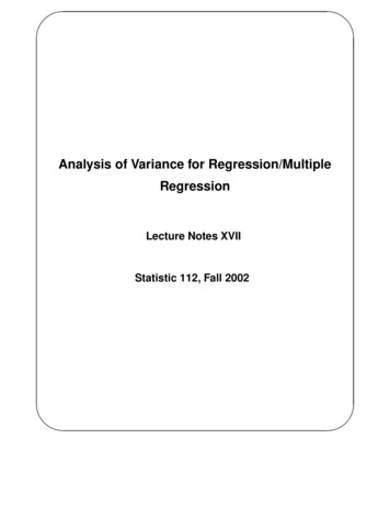
REGRESSION MODELS WITH ORDINAL VARIABLES1980). These methods, however, while elegantand well grounded in statistical theory, are difficult to use in the cases where regressionanalysis and its extensions would otherwiseapply: that is, where data are nontabular; include continuous, discrete, and ordinal variables; and apply to a causal model with severalendogenous variables.This article draws attention to alternativemethods for estimating regression models andtheir generalizations that include ordinal variables. These methods are extensions of logitand probit models for dichotomous variablesand are based on models that include unmeasured continuous variables for which only ordinal measures are available. Largely ignoredin the sociological literature (though seeMcKelvey and Zavoina, 1975), they providemultivariate models with ordinal variables that:(1) take account of noninterval ordinal measurement; (2) avoid arbitrary assumptionsabout the scale of ordinal variables; and, mostimportantly, (3) include ordinal variables instructural equation models with variables at alllevels of measurement. The ordered probit andlogit models can, moreover, be implementedwith widely available statistical software. Mostof the literature on these methods focuses onestimating equations with ordinal dependent1957;and Silvey,variables (AitchisonAmemiya, 1975; Ashford, 1959; Cox, 1970;Gurland et al., 1960; Maddala, 1983; McCullagh, 1980; McKelvey and Zavoina 1975),though some of it is relevant to models withordinal independent variables (Heckman, 1978;Winship and Mare, 1983). Taken together,these contributions imply that ordinal variablescan be analyzed within structural equationmodels with the same flexibility and power thatare available for continuous variables.This article summarizes the probit and logitmodels for ordered variables. It describes measurement models for ordinal variables and discusses specification and estimation of modelswith ordinal dependent and independent variables. Then it discusses some tests for modelmisspecification. Finally, it presents an empirical example which illustrates the models.An appendix discusses several technical topicsof interest to those who wish to implement themodels.MEASUREMENT OF ORDINALVARIABLESA common view of ordinal variables, which isadopted here, is that they are nonstrictmonotonic transformations of interval variables (e.g., O'Brien, 1981). That is, one ormore values of an interval-level variable aremapped into the same value of a transformed,513ordinal variable. For example, a Likert scalemay place individuals in one of a number ofranked categories, such as, "strongly agree,""somewhat agree," "neither agree nor disagree," "somewhat disagree," or "stronglydisagree" with a statement. An underlying,continuous variable denoting individuals' degrees of agreement is mapped into categoriesthat are ordered but are separated by unknowndistances. IThis view of ordinal variables can also applyto variables that are often treated as continuous but might be better viewed as ordinal.Counted variables, such as grades of schoolcompleted, number of children ever born, ornumber of voluntary-association memberships,may be regarded as ordinal realizations of underlying continuous variables. Grades ofschool, for example, should be viewed as anordinal measure of an underlying variable,"educational attainment," when one wishes toacknowledge that each grade is not equallyeasy to attain (e.g., Mare, 1980) or equallyrewarding (e.g., Featherman and Hauser, 1978;Jencks et al., 1979). Similarly, when a continuous variable, such as earnings, is measured incategories corresponding to dollar intervalsand category midpoints are unknown, the measured variable is an ordinal representation ofan underlying continuous variable.2The measurement model of ordinal variablescan be stated formally as follows. Let Y denotean unobserved, continuous variable (-w Y o) and a0, al, . . a, J-1, aj denote cut-pointsin the distribution of Y, where a0 - x andaj ? (see Figure 1). Let Y* be an ordinalvariable such thatY ajj if aj-,y (j 1,.,J).I A less common type of ordinal variable, not discussed further inithis article, may result from a strictmonotonic transformation of an interval variable.That is, observations (e.g., of cities, persons, occupations, etc.) may be ranked according to some unmeasured criterion (e.g., population size, wealth,rate of pay, etc.). A regression model with a rankeddependent variable requires that the nonlinear mapping between the unmeasured continuous rankingvariable and the ranks themselves be specified.Given the mapping, the model can be estimated bynonlinear least squares (e.g., Gallant, 1975).2 The ordinal-variable model can be extended totake account of measurement error. That is, an ordinal variable is a transformation of a continuous variable, but some observations may be misclassified(O'Brien, 1981; Johnson and Creech, 1983). Although this article does not discuss this complication, it is a logical extension of the models presentedhere. Muthen (1979), Avery and Hotz (1982), andWinship and Mare (1983) discuss this extension fordichotomous variables; Muthen (1983, 1984) discusses it for ordinal variables.
514AMERICAN SOCIOLOGICAL REVIEWindependent variables on an ordinal dependentvariable. The following discussion assumes asingle independentvariable,although- J) -F( /(Y)equations with several independent variablesare an obvious extension. For the iPh observation, let Yi be the unobserved continuous dependent variable Y (i 1,. . ., N), Xi be an1jJ-1j-1observed independent variable (which may beFigure 1. RelationshipsAmong Latent Continuous either continuous or dichotomous), Ei be a ranVariable (Y), Observed OrdinalVariable domly distributed error that is uncorrelated(Y*), and Thresholds(aj)with X, and l3 be a slope parameter to be estimated, Further, let YtIbe the observed ordinalSince Y is not observed, its mean and variance variable where, as in the measurement modelare unknown and their values must be as- above, Yi j if aj-, - Yi aj (j 1,.J).sumed. For the present, assume that Y has Then a regression model ismean of zero and variance of one.The relationship between Y and Y* can be EiYi 8xifurther understood as follows. Consider the(E(Y) ,3X; Var (Y) 1).(3)likelihood of obtaining a particular value of Yand the probability that Y* takes on a specificTo specify the model fully, it is necessary tovalue (see Figure 1). If Y follows a probability select a probability distribution for Y, ordistribution (for example, normal) with density equivalently for E. If the probability that Y*function f(Y) and cumulative density function takes on successively higher values rises (orF(Y), then the probability that Y* j is the falls) slowly at small values of X, more rapidlyarea under the density curve f(Y) between aj-1 for intermediate values of X, and more slowlyand aj. That is,again at large values of X, then either the normal or logistic distribution is appropriate for E.aiThe former distribution yields the ordered pro(1) bit model; the latter the ordered logit model.3P(Y* j) ff(Y)dy F(aj)-F(aj ),In contrast, a linear model, in which the unobwhere F(aj) 1 and F(a0) 0. For a sample ofserved variable Yi is replaced by the observedindividuals for whom Y* is observed one can ordinal variable Y* in the regression model,estimate the cutpoints or "thresholds" aj asassumes that the probability that Y* takes successively higher values rises (falls) a constantamount over the entire range of X.&j F-I(pj),When Y* takes on only two values, then (3)where pj is the proportion of observations for reduces to a model for a dichotomous depenwhich Y* j, and F-1 is the inverse of the dent variable and the alternative assumptionscumulative density function of Y. Given esti- of normal or logistic distributions yield binarymates of the aj, it is also possible to estimate probit and logit models respectively. Replacingthe mean of Y for observations within each the unobserved Yi with the observed binaryinterval. If Y follows a standardized normal variable yields a linear probability model. As isdistribution, then the mean Y for the observa- well known, the probit or logit specificationstions for which Y* j isare usually preferable to the linear model because the former take account of the ceilingand floor effects on the dependent variablek(a-j- 1)- (ai),(2) whereas the linear model does not (e.g.,Yaj, aji Hanushek and Jackson, 1977). When Y* is ordinal and takes on more than two values, thewhere 4 is the standardized normal probability ordered probit and logit models have a similardensity function and 1 is the cumulative stan- advantage over the linear regression model.dardized normal density function (Johnson and Whereas the former take account of ceiling andKotz, 1970).floor restrictions on the probabilities, the linearmodel does not. This advantage of the orderedprobit and logit over the linear model isstrongest when Y* is highly skewed or whenMODELS WITH ORDINAL DEPENDENTtwo or more groups with widely varyingVARIABLESf(Y)Model SpecificationGiven the measurement model for ordinal variables, it is possible to model the effects of3 Other models for binary dependent variables thatcan be extended to ordinal variables are discussedby, for example, Cox (1970) and McCullagh (1980).
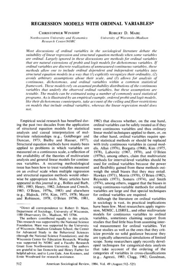
REGRESSION MODELS WITH ORDINAL VARIABLESskewness in Y* are compared (see examplebelow). The assumptionthat E follows a normalor logistic distribution,however, while oftenplausible, may be false. As discussed below,one can test this assumptionand, in principle,modifythe model to take account of departuresfrom the assumed distribution.EstimationIn practice, one seeks to estimate the slopeparameter(s)/3 and the threshold parametersa1, - . , aj-1.The formerdenotes the effect of aunit change in the independentvariable X onthe unobservedvariableY. The latter provideinformation about the distribution of theordered dependent variable such as whetherthe categories of the variable are equallyspaced in the probitor logit scale. Because theorderedprobit and logit models are nonlinear,exact algebraic expressions for their parameters do not exist. Instead, to compute the parameters, iterative estimation methods are required. This section summarizes the logic ofmaximumlikelihoodestimationfor these models as well as a useful non-maximumlikelihoodapproach. Furthertechnical details, includinginformationabout computersoftware, are presented in the Appendix.4Maximum Likelihood. If the unobserved de-pendentvariableY has conditionalexpectationgiven the independentvariables) E(YIX) ,3Xand varianceone, then the measurementmodel(1) can be modifiedto give the probabilitythatthe ith individualtakes the valuej on the ordinaldependent variable asp(Y* jjXj) -F(aj - 83Xj)F(a-1 - /3X1),(4)where F(ao - 83X1) 0 and F(aj - 83X1) 1because a0 -w and aj x. If the model is anorderedprobit, then F is the cumulativestandardnormaldensityfunction.If the modelis anorderedlogit, then F is the cumulativelogisticfunction. The quantities (4) for each individualare combinedto form the sample likelihood asfollows:L L1J7Ip(Y*i j1Xi)dij(5)iijwhere dijis a variablethat equals one if Yli i,and zero otherwise. Maximumlikelihood esti4Modelswith ordinal dependent variables canalso be estimated by weighted nonlinear leastsquares (e.g., Gurland et al., 1960). For modelsbased on distributions within the exponential family,such as the logit and probit, weighted nonlinear leastsquares and maximum likelihood estimation areequivalent (e.g., Nelder and Wedderburn, 1972;Bradley, 1973; Jennrich and Moore, 1975).515mationconsists of findingvalues of ,3and the ajin (4) that make L as large as possible.BinaryProbitor Logit.In practice,maximumlikelihoodestimationof the orderedlogit or probit model can be expensive, especially when the numbers of observations,thresholds, or independentvariables are largeand the analyst does not know what values ofthe unknown parameters would be suitable"start values" for the estimation. Moreover,although the ordered models can be implemented with widely available computersoftware (see Appendix),such applicationsareharderto masterand apply routinelythanmoreelementary methods. Other methods of estimation are cheaper and easier to use and consistently (though not efficiently) estimate theunknownparameters.These methods are useful both for exploratoryresearch where manymodels may be estimatedand for obtaininginitial values for maximumlikelihoodestimation.One method is to collapse the categories ofY* into a dichotomy, Y* j versus Y* - j,say, and to estimate (3) as a binary probit orlogit by the maximum likelihood methodsavailablein many statisticalpackagesor, if thedata are grouped, by weighted least squares(e.g., Hanushek and Jackson, 1977). Thisyields consistent estimates of /3 and of ai,though not of the remainingthresholds. Thismethod can also be appliedJ-1 times, once foreach of the J-1 splits between adjacentcategoriesof Y*, to estimateall of the as's, butthis yields J-1 estimates of /3, none of whichuses all of the informationin the data.A better alternative is to estimate the J-1binary logits or probits simultaneouslyto obtain estimates of the J-1 thresholdsand a common slope parameter,3. To do this, replicatethe data matrixJ-1 times, once for each of theJ-1 splits between adjacentcategoriesof Y*, toget a data set with (J-l)N observations. Eachof the J-1 data matrices has a differentcodingof the dependent variable to denote that anobservation is above or below the thresholdthat matrix estimates, and J-1 additionalcolumns are added to the matrix for J-1 dummyvariables, denoting which threshold is estimatedin each of the J-1 data sets. This methodis illustrated in Figure 2, which presents ahypotheticaldata matrixfor a dependentvariable having 4 ordered categories. The totalmatrixhas 3N observations.For clarity, withineach of the 3 replicates of the data, observations are orderedin ascendingorderof Y*. Thethird column denotes the dependent variablefor a binary logit or probit model, which iscoded one if the observation is above thethreshold and zero otherwise. In the firstpanel, observations scoring 2 or above on Y*have a one on the dependent variable; in the
516VariableAMERICAN SOCIOLOGICAL a331A0000X11X 0001141001Figure 2. Hypothetical Data Matrix for Dichotomous Estimation of Ordered Logit or Probit Model.second, observationsscoring3 or above on Y*have a one; and in the third, observationsscoring4 have a one. The fourththroughsixthcolumns denote which of the three thresholdsare estimated in each of the panels of the datamatrix.These are effect coded and thus can allbe included as independent variables in theprobit or logit model to estimate the threethresholds. The final two columns denote twoindependent variables, values of which arereplicatedexactly across the three panels.Althoughthis method requiresa largerdataset, it is a flexible way of exploringthe dataandobtaining preliminary estimates of the aj'sand /3's for maximum likelihood estimation.Estimates obtained by this method are oftenvery close to the maximum likelihood esti-mates (within 10 percent). The standarderrorsof the parameters are somewhat underestimated because the method assumes that thereare (J-1)N observations when only N areunique. In practice, however, this bias is oftensmall.5I In the probit model, the rationale for this methodis as follows: An ordered probit is equivalent to J- 1binary probits in which constants (thresholds) differ,slopes are identical (within variables acrossequations), and correlations among the disturbancesof the J- 1 equations are all equal to one. A binaryprobit estimated over J- 1 replicates of the data asdescribed here is equivalent to J- 1 binary probitswith varying constants and identical slopes but withdisturbance correlations all equal to zero. In practice, the slope and threshold estimates are insensitive
517REGRESSION MODELS WITH ORDINAL VARIABLESScaling of CoefficientsMost computer programs for ordered probit orlogit estimation fix the variance of E at I in theprobit model or at ir2/3 in the logit model ratherthan fix the variance of Y as in (3) above.Although computationally efficient, this practice may lead to ambiguous comparisons between the coefficients of different equations.Adding new independent variables to an equation alters the variance of Y and thus the remaining coefficients in the model, even if thenew independent variables are uncorrelatedwith the original independent variables. Whenestimating several equations with a commonordinal dependent variable it is advisable torescale estimated coefficients to a constantvariance for the latent dependent variable (sayVar(Y) 1) across equations. The resultingcoefficients will then measure the change instandard deviations in the latent continuousvariable per unit changes in the independentvariables.If, for example, the computations assumethat Var(E) 1 but Var(Y) 1, then the estimated equation isYi bXi eiwhere b 1(3E1E,ei Ei/o-E, and Var(E) v .Then roI 1/[1 b2Var(X)] and ,3 boa.Under this scaling assumption, oe decreases asadditional variables that affect Y are includedin the equation, and measures the proportion ofvariance in Y that is unexplained by the independent variables. Thus 1 - o-2 is analogous toR2 in a linear regression.MODELS WITH ORDINALINDEPENDENT VARIABLESOrdinal variables may also be independent orintervening variables in structural equationmodels. For example, job tenure, a continuousvariable, may depend on job satisfaction, anordinal variable measured on a Likert scale, aswell as on other variables. Job satisfaction inturn may depend on characteristics of individuals and their jobs. One solution to this problem is to assume that the ordered categoriesconstitute a continuous scale, but this is inappropriate if the ordered variable Y* is nonlinearly related to an unobserved continuousvariable Y (as in the model discussed above)and it is the unobserved variable that linearlyaffects the dependent variable. Another strategy is to represent Y* as J- 1 dummy variablesand to estimate their effects on the dependentto alternative assumptions about the disturbancecorrelations.variable. This strategy, however, is unparsimonious, fails to use the information that thecategories of Y* are ordered, and may stillyield biased estimates if the correct model is alinear effect of the unobserved variable Y onthe dependent variable. This section considersseveral preferable solutions to this problem.Consider the following two equations:Zi 31X1i f32Yi EziYi 01X1i 02X2i Eyi(6)(7)where for the ith observation Z is continuousand may be either an observed variable or anunobserved variable that corresponds to an observed dichotomous or ordinal variable, sayZ*; Y is an unobserved continuous variablecorresponding to an observed ordinal variableY* through the measurement model discussedabove; X1 and X2 are observed continuous ordichotomous variables; ez and Ey are randomerrors that are uncorrelated with each otherand with their respective independent variables; and the ,3's and 0's are parameters to beestimated. If this model is correct, that is, if theeffect of the ordinal variable Y* on Z is properly viewed as the linear effect of the observedvariable Y, of which Y* is a realization, thenseveral methods of identifying and estimating/32 are available. These methods include: (1)instrumental-variable estimation; (2) estimation based on the conditional distribution of Y;and (3) maximum likelihood estimation. Thesemethods are summarized in turn.Instrumental VariablesOne method of estimating (6) and (7) is to usethe fact that X2 affects Y but not Z, that is, thatX2 is an instrumental variable for Y. First, estimate (7) as an ordered logit or probit modelby the procedures discussed above and, usingthe estimated equation, calculate expectedvalues for Y:E(YjjXjj, X20) Yi 61X1i 62X2i.Then, in a second stage of estimation, replaceY with Y in (6) and estimate the latter equationby a method suited to the measurement of Z(ordinary least squares (OLS), probit, logit,etc.). This method consistently estimates /3'and /2 under the assumption that Ezand Ey areuncorrelated with each other and with X, andX2. Standard errors for estimated parameters6 A fourth method is to rely on multiple indicatorsof Y, as would be possible if, for example, Y denotedjob satisfaction and Ye and Y* were Likert scales ofsatisfaction with specific aspects of a job (pay, opportunity for advancement, etc.).
518AMERICAN SOCIOLOGICAL REVIEWshould be computed using the usual formulasfor instrumental-variable estimation (e.g.,Johnston, 1972:280).This method works only if X2 affects Y butnot Z; otherwise Y would be an exact linearcombinationof variablesalready in (6) and 32would not be estimable. In addition, for themethod to yield precise estimates, X2 and Yshould be strongly associated. When theseconditions are not met, alternative methodsshould be considered.Using the Conditional Distribution of YIf Z is an observed continuousvariable,and Zand Y follow a bivariatenormal distribution,then an alternativemethodof estimatingY forsubstitutionin (6) is available.Suppose 02 0,that is, there is no instrumentalvariable X2through which to identify /2 in (6). One cannonethelesscomputeexpected values of Y thatare not linearly dependenton variables in (6)by using the relationshipbetween Y and Y*:E(YilXli, lx1,Y*) Yi 4(&?i (D(a'j-01X1i E(YyiXli, Y*)1X1i) 01X11)-(c(a?i 1- 01X1-lXi))tion, (6) and (7) can be estimated simultaneously regardless of whether Z results froman observed continuous or ordinal variable.Suppose that 02 0 in (7), that is, that there isno instrumentalvariable and that Var(E,) Var(E,) 1. (Maximum likelihood, like themethodbased on the conditionalexpectationofY, works regardlessof whether 02 0.) Thenthe reduced form of (6) isZi where 8, aiX1i Vi(9) 32EYi, andThe maximumlikelihood procedure estimates (7) and (9) simultaneouslyalong with p. Thus 01, 02, and /2are estimateddirectly, and 8,3can be calculatedas 81 - 201.-7The estimation procedure itself consists ofcomputingthe joint probabilitiesof obtainingZ(or Z* if Z is an unobservedvariablefor whichonly an ordinalvariableis observed)and Y* foreach individual and forming the likelihoodwhich, assuming a bivariate normal distribution for Z and Y, dependson the reduced-formparametersin (7) and (9) and on p. The methodsearches for values of the parameters thatmake the likelihood as large as possible. Seethe Appendix for furthertechnical details.COv(VEy) /31 P /3201,820,YVi Ezi32.where all parametersare taken from orderedprobitestimatesof (7) (excludingX2). The sec- Extensionsond term in (8) is an extention of equation (2) Given estimatesof equationsthat include ordiabove to the case whereeach observationhas a nal variables as either dependent or indepenmean conditionalon its.value of X1 in addition dent variables, it is possible to formulateto Y*. With predicted values Y in hand, onestructural equation models with mixtures ofcan then substitutethem for Y in (6) and esti- continuous, discrete and ordinalvariables. Asmatethatequationby least-squaresregression. a result one can compute direct and indirectThis method is a variant of procedures for effects of exogenous variableson ultimateenestimating regression equations that are sub- dogenous variableseven when the interveningject to "sample selection bias" (Berk, 1983; variablesare ordinal.The same proceduresdeHeckman, 1979). It permits identification of scribed by Winshipand Mare (1983:82-86)forthe effects of the unmeasuredvariableY in (6) the path analysis of dichotomousvariablescanin the absence of the instrumentalvariableX2 be applied to systems in which some of thebecause it takes account of the correlation variables are ordinal.between Eyand the disturbanceof the reducedIn addition, the models described here canform of (6) (thatis, El 32EY), which is ignored be extended to allow for the discrete and conin the instrumental-variableestimation. This tinuous effects of ordinal variables. If, formethodrelies on the assumedbivariatenormal example, a continuousvariable, say, earnings,distribution of the disturbances of the two is affected by an ordinalvariable, say, highestequations. One should be cautious about the grade of school completed, one might elect todegree to which one's results may depend on model the school effect as twofold: (1) as anthis distributionalassumption.effect of a latent continuousvariable, "educational attainment";and (2) as the effect(s) ofattaining particular schooling milestones orMaximum LikelihoodEstimationIdentifying,/3 usingthe conditionaldistributionof Y requiresthat Z be an observedcontinuousvariable. It is not a fully efficient method inthat it relies on two separateestimationstages.If Z and Y follow a bivariatenormaldistribu-7If alternative assumptions about Var(E,) aidVar(E,) are made, the esti
with widely available statistical software. Most of the literature on these methods focuses on estimating equations with ordinal dependent variables (Aitchison and Silvey, 1957; Amemiya, 1975; Ashford, 1959; Cox, 1970; . ping between the unmeasured continuous ranking variable and the ranks themselves be specified. Given the mapping, the model .