Transcription
Statistical Analysis With Latent VariablesUser’s GuideLinda K. MuthénBengt O. Muthén
Following is the correct citation for this document:Muthén, L.K. and Muthén, B.O. (1998-2017). Mplus User’s Guide. Eighth Edition.Los Angeles, CA: Muthén & MuthénCopyright 1998-2017 Muthén & MuthénProgram Copyright 1998-2017 Muthén & MuthénVersion 8April 2017The development of this software has been funded in whole or in part with Federal fundsfrom the National Institute on Alcohol Abuse and Alcoholism, National Institutes ofHealth, under Contract No. N44AA52008 and Contract No. N44AA92009.Muthén & Muthén3463 Stoner AvenueLos Angeles, CA 90066Tel: (310) 391-9971Fax: (310) 391-8971Web: www.StatModel.comSupport@StatModel.com
TABLE OF CONTENTSChapter 1: Introduction1Chapter 2: Getting started with Mplus13Chapter 3: Regression and path analysis19Chapter 4: Exploratory factor analysis43Chapter 5: Confirmatory factor analysis and structural equation modeling55Chapter 6: Growth modeling, survival analysis, and N 1 time series analysis113Chapter 7: Mixture modeling with cross-sectional data165Chapter 8: Mixture modeling with longitudinal data221Chapter 9: Multilevel modeling with complex survey data261Chapter 10: Multilevel mixture modeling395Chapter 11: Missing data modeling and Bayesian analysis443Chapter 12: Monte Carlo simulation studies465Chapter 13: Special features499Chapter 14: Special modeling issues515Chapter 15: TITLE, DATA, VARIABLE, and DEFINE commands563Chapter 16: ANALYSIS command651Chapter 17: MODEL command711Chapter 18: OUTPUT, SAVEDATA, and PLOT commands791Chapter 19: MONTECARLO command859Chapter 20: A summary of the Mplus language893
PREFACEWe started to develop Mplus in 1995 with the goal of providing researchers withpowerful new statistical modeling techniques. We saw a wide gap between newstatistical methods presented in the statistical literature and the statistical methods usedby researchers in substantively-oriented papers. Our goal was to help bridge this gapwith easy-to-use but powerful software. Version 1 of Mplus was released in November1998; Version 2 was released in February 2001; Version 3 was released in March 2004;Version 4 was released in February 2006; Version 5 was released in November 2007,Version 6 was released in April 2010; and Version 7 was released in September 2012.After four expansions of Version 7 during the last five years, we are now proud to presentthe new and unique features of Version 8. With Version 8, we have gone a considerableway toward accomplishing our goal, and we plan to continue to pursue it in the future.The new features that have been added between Version 7 and Version 8 would neverhave been accomplished without two very important team members, TihomirAsparouhov and Thuy Nguyen. It may be hard to believe that the Mplus team has onlytwo programmers, but these two programmers are extraordinary. Tihomir has developedand programmed sophisticated statistical algorithms to make the new modeling possible.Without his ingenuity, they would not exist. His deep insights into complex modelingissues and statistical theory are invaluable. Thuy has developed the post-processinggraphics module, the Mplus editor and language generator, and the Mplus Diagrammerbased on a framework designed by Delian Asparouhov. In addition, Thuy hasprogrammed the Mplus language and is responsible for producing new release versions,testing, and keeping control of the entire code which has grown enormously. Herunwavering consistency, logic, and steady and calm approach to problems keep everyoneon target. We feel fortunate to work with such a talented team. Not only are theyextremely bright, but they are also hard-working, loyal, and always striving forexcellence. Mplus Version 8 would not have been possible without them.Another important team member is Michelle Conn. Michelle was with us at thebeginning when she was instrumental in setting up the Mplus office and returned fifteenyears ago. Michelle wears many hats: Chief Financial Officer, Office Manager, andSales Manager, among others. She was the driving force behind the design of the newshopping cart. With the vastly increased customer base, her efficiency in multi-taskingand calm under pressure are much appreciated. Noah Hastings joined the Mplus team in2009. He is responsible for testing the Graphics Module and the Mplus Diagrammer,creating the pictures of the models in the example chapters of the Mplus User’s Guide,
keeping the website updated, and providing assistance to Bengt with presentations,papers, and our book. He has proven to be a most trustworthy and valuable teammember.We would also like to thank all of the people who have contributed to the development ofMplus in past years. These include Stephen Du Toit, Shyan Lam, Damir Spisic, KerbyShedden, and John Molitor.Initial work on Mplus was supported by SBIR contracts and grants from NIAAA that weacknowledge gratefully. We thank Bridget Grant for her encouragement in this work.Linda K. MuthénBengt O. MuthénLos Angeles, CaliforniaApril 2017
IntroductionCHAPTER 1INTRODUCTIONMplus is a statistical modeling program that provides researchers with aflexible tool to analyze their data. Mplus offers researchers a widechoice of models, estimators, and algorithms in a program that has aneasy-to-use interface and graphical displays of data and analysis results.Mplus allows the analysis of both cross-sectional and longitudinal data,single-level and multilevel data, data that come from differentpopulations with either observed or unobserved heterogeneity, and datathat contain missing values. Analyses can be carried out for observedvariables that are continuous, censored, binary, ordered categorical(ordinal), unordered categorical (nominal), counts, or combinations ofthese variable types. In addition, Mplus has extensive capabilities forMonte Carlo simulation studies, where data can be generated andanalyzed according to most of the models included in the program.The Mplus modeling framework draws on the unifying theme of latentvariables. The generality of the Mplus modeling framework comes fromthe unique use of both continuous and categorical latent variables.Continuous latent variables are used to represent factors correspondingto unobserved constructs, random effects corresponding to individualdifferences in development, random effects corresponding to variation incoefficients across groups in hierarchical data, frailties corresponding tounobserved heterogeneity in survival time, liabilities corresponding togenetic susceptibility to disease, and latent response variable valuescorresponding to missing data. Categorical latent variables are used torepresent latent classes corresponding to homogeneous groups ofindividuals, latent trajectory classes corresponding to types ofdevelopment in unobserved populations, mixture componentscorresponding to finite mixtures of unobserved populations, and latentresponse variable categories corresponding to missing data.THE Mplus MODELING FRAMEWORKThe purpose of modeling data is to describe the structure of data in asimple way so that it is understandable and interpretable. Essentially,the modeling of data amounts to specifying a set of relationships1
CHAPTER 1between variables. The figure below shows the types of relationshipsthat can be modeled in Mplus. The rectangles represent observedvariables. Observed variables can be outcome variables or backgroundvariables. Background variables are referred to as x; continuous andcensored outcome variables are referred to as y; and binary, orderedcategorical (ordinal), unordered categorical (nominal), and countoutcome variables are referred to as u. The circles represent latentvariables. Both continuous and categorical latent variables are allowed.Continuous latent variables are referred to as f. Categorical latentvariables are referred to as c.The arrows in the figure represent regression relationships betweenvariables. Regressions relationships that are allowed but not specificallyshown in the figure include regressions among observed outcomevariables, among continuous latent variables, and among categoricallatent variables. For continuous outcome variables, linear regressionmodels are used. For censored outcome variables, censored (tobit)regression models are used, with or without inflation at the censoringpoint. For binary and ordered categorical outcomes, probit or logisticregressions models are used. For unordered categorical outcomes,multinomial logistic regression models are used. For count outcomes,Poisson and negative binomial regression models are used, with orwithout inflation at the zero point.2
IntroductionModels in Mplus can include continuous latent variables, categoricallatent variables, or a combination of continuous and categorical latentvariables. In the figure above, Ellipse A describes models with onlycontinuous latent variables. Ellipse B describes models with onlycategorical latent variables. The full modeling framework describesmodels with a combination of continuous and categorical latentvariables. The Within and Between parts of the figure above indicatethat multilevel models that describe individual-level (within) and clusterlevel (between) variation can be estimated using Mplus.MODELING WITH CONTINUOUS LATENTVARIABLESEllipse A describes models with only continuous latent variables.Following are models in Ellipse A that can be estimated using Mplus:3
CHAPTER 1 Regression analysisPath analysisExploratory factor analysisConfirmatory factor analysisItem response theory modelingStructural equation modelingGrowth modelingDiscrete-time survival analysisContinuous-time survival analysisTime series analysisObserved outcome variables can be continuous, censored, binary,ordered categorical (ordinal), unordered categorical (nominal), counts,or combinations of these variable types.Special features available with the above models for all observedoutcome variables types are: 4Single or multiple group analysisMissing data under MCAR, MAR, and NMAR and with multipleimputationComplex survey data features including stratification, clustering,unequal probabilities of selection (sampling weights), subpopulationanalysis, replicate weights, and finite population correctionLatent variable interactions and non-linear factor analysis usingmaximum likelihoodRandom slopesIndividually-varying times of observationsLinear and non-linear parameter constraintsIndirect effects including specific pathsMaximum likelihood estimation for all outcomes typesBootstrap standard errors and confidence intervalsWald chi-square test of parameter equalitiesFactor scores and plausible values for latent variables
IntroductionMODELING WITH CATEGORICAL LATENTVARIABLESEllipse B describes models with only categorical latent variables.Following are models in Ellipse B that can be estimated using Mplus: Regression mixture modeling Path analysis mixture modeling Latent class analysis Latent class analysis with covariates and direct effects Confirmatory latent class analysis Latent class analysis with multiple categorical latent variables Loglinear modeling Non-parametric modeling of latent variable distributions Multiple group analysis Finite mixture modeling Complier Average Causal Effect (CACE) modeling Latent transition analysis and hidden Markov modeling includingmixtures and covariates Latent class growth analysis Discrete-time survival mixture analysis Continuous-time survival mixture analysisObserved outcome variables can be continuous, censored, binary,ordered categorical (ordinal), unordered categorical (nominal), counts,or combinations of these variable types. Most of the special featureslisted above are available for models with categorical latent variables.The following special features are also available. Analysis with between-level categorical latent variablesTests to identify possible covariates not included in the analysis thatinfluence the categorical latent variablesTests of equality of means across latent classes on variables notincluded in the analysisPlausible values for latent classes5
CHAPTER 1MODELING WITH BOTH CONTINUOUS ANDCATEGORICAL LATENT VARIABLESThe full modeling framework includes models with a combination ofcontinuous and categorical latent variables. Observed outcome variablescan be continuous, censored, binary, ordered categorical (ordinal),unordered categorical (nominal), counts, or combinations of thesevariable types. Most of the special features listed above are available formodels with both continuous and categorical latent variables. Followingare models in the full modeling framework that can be estimated usingMplus: Latent class analysis with random effectsFactor mixture modelingStructural equation mixture modelingGrowth mixture modeling with latent trajectory classesDiscrete-time survival mixture analysisContinuous-time survival mixture analysisMost of the special features listed above are available for models withboth continuous and categorical latent variables. The following specialfeatures are also available. Analysis with between-level categorical latent variablesTests to identify possible covariates not included in the analysis thatinfluence the categorical latent variablesTests of equality of means across latent classes on variables notincluded in the analysisMODELING WITH COMPLEX SURVEY DATAThere are two approaches to the analysis of complex survey data inMplus. One approach is to compute standard errors and a chi-square testof model fit taking into account stratification, non-independence ofobservations due to cluster sampling, and/or unequal probability ofselection.Subpopulation analysis, replicate weights, and finitepopulation correction are also available. With sampling weights,parameters are estimated by maximizing a weighted loglikelihoodfunction. Standard error computations use a sandwich estimator. Forthis approach, observed outcome variables can be continuous, censored,6
Introductionbinary, ordered categorical (ordinal), unordered categorical (nominal),counts, or combinations of these variable types.A second approach is to specify a model for each level of the multileveldata thereby modeling the non-independence of observations due tocluster sampling. This is commonly referred to as multilevel modeling.The use of sampling weights in the estimation of parameters, standarderrors, and the chi-square test of model fit is allowed. Both individuallevel and cluster-level weights can be used. With sampling weights,parameters are estimated by maximizing a weighted loglikelihoodfunction. Standard error computations use a sandwich estimator. Forthis approach, observed outcome variables can be continuous, censored,binary, ordered categorical (ordinal), unordered categorical (nominal),counts, or combinations of these variable types.The multilevel extension of the full modeling framework allows randomintercepts and random slopes that vary across clusters in hierarchicaldata. Random slopes include the special case of random factor loadings.These random effects can be specified for any of the relationships of thefull Mplus model for both independent and dependent variables and bothobserved and latent variables. Random effects representing acrosscluster variation in intercepts and slopes or individual differences ingrowth can be combined with factors measured by multiple indicators onboth the individual and cluster levels. In line with SEM, regressionsamong random effects, among factors, and between random effects andfactors are allowed.The two approaches described above can be combined. In addition tospecifying a model for each level of the multilevel data therebymodeling the non-independence of observations due to cluster sampling,standard errors and a chi-square test of model fit are computed takinginto account stratification, non-independence of observations due tocluster sampling, and/or unequal probability of selection. When there isclustering due to both primary and secondary sampling stages, thestandard errors and chi-square test of model fit are computed taking intoaccount the clustering due to the primary sampling stage and clusteringdue to the secondary sampling stage is modeled.Most of the special features listed above are available for modeling ofcomplex survey data.7
CHAPTER 1MODELING WITH MISSING DATAMplus has several options for the estimation of models with missingdata. Mplus provides maximum likelihood estimation under MCAR(missing completely at random), MAR (missing at random), and NMAR(not missing at random) for continuous, censored, binary, orderedcategorical (ordinal), unordered categorical (nominal), counts, orcombinations of these variable types (Little & Rubin, 2002). MARmeans that missingness can be a function of observed covariates andobserved outcomes. For censored and categorical outcomes usingweighted least squares estimation, missingness is allowed to be afunction of the observed covariates but not the observed outcomes(Asparouhov & Muthén, 2010a). When there are no covariates in themodel, this is analogous to pairwise present analysis. Non-ignorablemissing data (NMAR) modeling is possible using maximum likelihoodestimation where categorical outcomes are indicators of missingness andwhere missingness can be predicted by continuous and categorical latentvariables (Muthén, Jo, & Brown, 2003; Muthén et al., 2011).In all models, missingness is not allowed for the observed covariatesbecause they are not part of the model. The model is estimatedconditional on the covariates and no distributional assumptions are madeabout the covariates. Covariate missingness can be modeled if thecovariates are brought into the model and distributional assumptionssuch as normality are made about them. With missing data, the standarderrors for the parameter estimates are computed using the observedinformation matrix (Kenward & Molenberghs, 1998). Bootstrapstandard errors and confidence intervals are also available with missingdata.Mplus provides multiple imputation of missing data using Bayesiananalysis (Rubin, 1987; Schafer, 1997). Both the unrestricted H1 modeland a restricted H0 model can be used for imputation. Multiple data setsgenerated using multiple imputation can be analyzed using a specialfeature of Mplus. Parameter estimates are averaged over the set ofanalyses, and standard errors are computed using the average of thestandard errors over the set of analyses and the between analysisparameter estimate variation (Rubin, 1987; Schafer, 1997). A chi-squaretest of overall model fit is provided (Asparouhov & Muthén, 2008c;Enders, 2010).8
IntroductionESTIMATORS AND ALGORITHMSMplus provides both Bayesian and frequentist inference. Bayesiananalysis uses Markov chain Monte Carlo (MCMC) algorithms. Posteriordistributions can be monitored by trace and autocorrelation plots.Convergence can be monitored by the Gelman-Rubin potential scalingreduction using parallel computing in multiple MCMC chains. Posteriorpredictive checks are provided.Frequentist analysis uses maximum likelihood and weighted leastsquares estimators. Mplus provides maximum likelihood estimation forall models. With censored and categorical outcomes, an alternativeweighted least squares estimator is also available. For all types ofoutcomes, robust estimation of standard errors and robust chi-squaretests of model fit are provided. These procedures take into account nonnormality of outcomes and non-independence of observations due tocluster sampling. Robust standard errors are computed using thesandwich estimator. Robust chi-square tests of model fit are computedusing mean and mean and variance adjustments as well as a likelihoodbased approach. Bootstrap standard errors are available for mostmodels. The optimization algorithms use one or a combination of thefollowing: Quasi-Newton, Fisher scoring, Newton-Raphson, and theExpectation Maximization (EM) algorithm (Dempster et al., 1977).Linear and non-linear parameter constraints are allowed.Withmaximum likelihood estimation and categorical outcomes, models withcontinuous latent variables and missing data for dependent variablesrequire numerical integration in the computations. The numericalintegration is carried out with or without adaptive quadrature incombination with rectangular integration, Gauss-Hermite integration, orMonte Carlo integration.MONTE CARLO SIMULATION CAPABILITIESMplus has extensive Monte Carlo facilities both for data generation anddata analysis. Several types of data can be generated: simple randomsamples, clustered (multilevel) data, missing data, discrete- andcontinuous-time survival data, and data from populations that areobserved (multiple groups) or unobserved (latent classes). Datageneration models can include random effects and interactions betweencontinuous latent variables and between categorical latent variables.Outcome variables can be generated as continuous, censored, binary,9
CHAPTER 1ordered categorical (ordinal), unordered categorical (nominal), counts,or combinations of these variable types.In addition, two-part(semicontinuous) variables and time-to-event variables can be generated.Independent variables can be generated as binary or continuous. All orsome of the Monte Carlo generated data sets can be saved.The analysis model can be different from the data generation model. Forexample, variables can be generated as categorical and analyzed ascontinuous or generated as a three-class model and analyzed as a twoclass model. In some situations, a special external Monte Carlo featureis needed to generate data by one model and analyze it by a differentmodel. For example, variables can be generated using a clustered designand analyzed ignoring the clustering. Data generated outside of Mpluscan also be analyzed using this special external Monte Carlo feature.Other special Monte Carlo features include saving parameter estimatesfrom the analysis of real data to be used as population and/or coveragevalues for data generation in a Monte Carlo simulation study. Inaddition, analysis results from each replication of a Monte Carlosimulation study can be saved in an external file.GRAPHICSMplus includes a dialog-based, post-processing graphics module thatprovides graphical displays of observed data and analysis resultsincluding outliers and influential observations.These graphical displays can be viewed after the Mplus analysis iscompleted. They include histograms, scatterplots, plots of individualobserved and estimated values, plots of sample and estimated means andproportions/probabilities, plots of estimated probabilities for acategorical latent variable as a function of its covariates, plots of itemcharacteristic curves and information curves, plots of survival andhazard curves, plots of missing data statistics, plots of user-specifiedfunctions, and plots related to Bayesian estimation. These are availablefor the total sample, by group, by class, and adjusted for covariates. Thegraphical displays can be edited and exported as a DIB, EMF, or JPEGfile. In addition, the data for each graphical display can be saved in anexternal file for use by another graphics program.10
IntroductionDIAGRAMMERThe Diagrammer can be used to draw an input diagram, to automaticallycreate an output diagram, and to automatically create a diagram using anMplus input without an analysis or data. To draw an input diagram, theDiagrammer is accessed through the Open Diagrammer menu option ofthe Diagram menu in the Mplus Editor. The Diagrammer uses a set ofdrawing tools and pop-up menus to draw a diagram. When an inputdiagram is drawn, a partial input is created which can be edited beforethe analysis. To automatically create an output diagram, an input iscreated in the Mplus Editor. The output diagram is automaticallycreated when the analysis is completed. This diagram can be edited andused in a new analysis. The Diagrammer can be used as a drawing toolby using an input without an analysis or data.LTA CALCULATORConditional probabilities, including latent transition probabilities, fordifferent values of a set of covariates can be computed using the LTACalculator. It is accessed by choosing LTA calculator from the Mplusmenu of the Mplus Editor.LANGUAGE GENERATORMplus includes a language generator to help users create Mplus inputfiles. The language generator takes users through a series of screens thatprompts them for information about their data and model. The languagegenerator contains all of the Mplus commands except DEFINE,MODEL, PLOT, and MONTECARLO. Features added after Version 2are not included in the language generator.THE ORGANIZATION OF THE USER’S GUIDEThe Mplus User’s Guide has 20 chapters. Chapter 2 describes how toget started with Mplus. Chapters 3 through 13 contain examples ofanalyses that can be done using Mplus. Chapter 14 discusses specialissues. Chapters 15 through 19 describe the Mplus language. Chapter20 contains a summary of the Mplus language. Technical appendicesthat contain information on modeling, model estimation, model testing,11
CHAPTER 1numerical algorithms, and references to further technical informationcan be found at www.statmodel.com.It is not necessary to read the entire User’s Guide before using theprogram. A user may go straight to Chapter 2 for an overview of Mplusand then to one of the example chapters.12
Getting Started With MplusCHAPTER 2GETTING STARTED WITH MplusAfter Mplus is installed, the program can be run from the Mplus editor.The Mplus Editor for Windows includes a language generator and agraphics module. The graphics module provides graphical displays ofobserved data and analysis results.In this chapter, a brief description of the user language is presentedalong with an overview of the examples and some model estimationconsiderations.THE Mplus LANGUAGEThe user language for Mplus consists of a set of ten commands each ofwhich has several options. The default options for Mplus have beenchosen so that user input can be minimized for the most common typesof analyses. For most analyses, only a small subset of the Mpluscommands is needed. Complicated models can be easily described usingthe Mplus language. The ten commands of Mplus are: PLOTMONTECARLO(required)(required)The TITLE command is used to provide a title for the analysis. TheDATA command is used to provide information about the data set to beanalyzed. The VARIABLE command is used to provide informationabout the variables in the data set to be analyzed. The DEFINEcommand is used to transform existing variables and create newvariables. The ANALYSIS command is used to describe the technical13
CHAPTER 2details of the analysis. The MODEL command is used to describe themodel to be estimated. The OUTPUT command is used to requestadditional output not included as the default. The SAVEDATAcommand is used to save the analysis data, auxiliary data, and a varietyof analysis results. The PLOT command is used to request graphicaldisplays of observed data and analysis results. The MONTECARLOcommand is used to specify the details of a Monte Carlo simulationstudy.The Mplus commands may come in any order. The DATA andVARIABLE commands are required for all analyses. All commandsmust begin on a new line and must be followed by a colon. Semicolonsseparate command options. There can be more than one option per line.The records in the input setup must be no longer than 90 columns. Theycan contain upper and/or lower case letters and tabs.Commands, options, and option settings can be shortened forconvenience. Commands and options can be shortened to four or moreletters. Option settings can be referred to by either the complete word orthe part of the word shown in bold type in the command boxes in eachchapter.Comments can be included anywhere in the input setup. A comment isdesignated by an exclamation point. Anything on a line following anexclamation point is treated as a user comment and is ignored by theprogram. Several lines can be commented out by starting the first linewith !* and ending the last line with *!.The keywords IS, ARE, and can be used interchangeably in allcommands except DEFINE, MODEL CONSTRAINT, and MODELTEST. Items in a list can be separated by blanks or commas.Mplus uses a hyphen (-) to indicate a list of variables or numbers. Theuse of this feature is discussed in each section for which it is appropriate.There is also a special keyword ALL which can be used to indicate allvariables. This keyword is discussed with the options that use it.Following is a set of Mplus input files for a few prototypical examples.The first example shows the input file for a factor analysis withcovariates (MIMIC model).14
Getting Started With MplusTITLE:this is an example of a MIMIC modelwith two factors, six continuous factorindicators, and three covariatesDATA:FILE IS mimic.dat;VARIABLE: NAMES ARE y1-y6 x1-x3;MODEL:f1 BY y1-y3;f2 BY y4-y6;f1 f2 ON x1-x3;The second example shows the input file for a growth model with timeinvariant covariates. It illustrates the new simplified Mplus language forspecifying growth models.TITLE:this is an example of a linear growthmodel for a continuous outcome at fourtime points with the intercept and slopegrowth factors regressed on two timeinvariant covariatesDATA:FILE IS growth.dat;VARIABLE: NAMES ARE y1-y4 x1 x2;MODEL:i s y1@0 y2@1 y3@2 y4@3;i s ON x1 x2;The third example shows the input file for a latent class analysis withcovariates and a direct effect.TITLE:this is an example of a latent classanalysis with two classes, one covariate,and a direct effectDATA:FILE IS lcax.dat;VARIABLE: NAMES ARE u1-u4 x;CLASSES c (2);CATEGORICAL u1-u4;ANALYSIS: TYPE MIXTURE;MODEL:%OVERALL%c ON x;u4 ON x;The fourth example shows the input file for a multilevel regressionmodel with a random intercept and a random slope varyi
creating the pictures of the models in the example chapters of the Mplus User's Guide, . latent variables. For continuous outcome variables, linear regression models are used. For censored outcome variables, censored (tobit) regression models are used, with or without inflation at the censoring . Missing data under MCAR, MAR, and NMAR and .