Transcription
Module 5 - Ordinal RegressionObjectives1. Understand the principles and theories underlying Ordinal Regression2. Understand the assumption of Proportional Odds and how to test it3. Be able to implement Ordinal Regression analyses using SPSS and accuratelyinterpret the output4. Be able to include interaction terms in your ordinal regression model and to accuratelyinterpret the output5. Appreciate the applications of Ordinal Regression in education research and thinkabout how it may be useful in your own researchStart Module 5: Ordinal RegressionUsing multiple variables to predict ordinal outcomes.You can jump to specific pages using the contents list below. If you are new to this modulestart at the Introduction and work through section by section using the 'Next' and 'Previous'buttons at the top and bottom of each page. Be sure to tackle the exercise and the quiz to geta good understanding.
Contents5.1Introduction5.2Working with ordinal outcomes5.3Key assumptions of ordinal regression5.4Example 1 - Running an ordinal regression on SPSS5.5Teacher expectations and tiering5.6Example 2 - Running an ordinal regression for mathematics tier of entry5.7Example 3 - Evaluating interaction effects in ordinal regression5.8Example 4 - Including a control for prior attainment5.9What to do if the assumption of proportional odds is not met?5.10Reporting the results of ordinal regression5.11ConclusionsQuizExercise
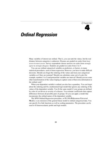
5.1 IntroductionIn previous modules we have seen how we can use linear regression to model a continuousoutcome measure (like age 14 test score), and also logistic regression to model a binaryoutcome (like achieving 5 GCSE A*-C passes). However you will remember from theFoundation Module that we typically define measures at three levels: nominal, ordinal andcontinuous. What we have not covered therefore is this „intermediate‟ level where ouroutcome is ordinal. You will remember that an ordinal measure includes information on rankordering within the data. For example we might have Likert scale measures such as “Howstrongly do you agree that you love statistics” which may be rated on a 5 point scale rangingfrom strongly disagree (1) to strongly agree (5). Another example is OFSTED (Office forStandards in Education) lesson evaluations which may be graded as „unsatisfactory‟,„satisfactory‟, „good‟ or „outstanding‟. Such examples are common in the social sciences.There are a number of ordinal outcomes in our LSYPE dataset. One is the KS3 (age 14)English test level. In England students‟ performance is recorded in terms of nationalcurriculum (NC) levels. These levels are reported on an age related scale, with the „typical‟student at age 7 expected to achieve level 2, at age 9 level 3, at age 11 level 4, and at age 14somewhere between level 5 and level 6. These levels may be determined through teacherassessment or be expressed as summaries from continuous test marks. Figure 5.1.1 showsthe distribution of students by English level from our dataset.Figure 5.1.1 Proportion of students at each English test levelWe do have access to the actual test marks in LSYPE, but often test marks are not availableand NC levels might be the only data recorded. In any event, this is a good example of an
ordinal outcome which we can work with to demonstrate the particular analyses that you canapply when your outcome measure is ordinal.The good news is that, bar a little extra work, the assumptions and concepts we need forordinal regression have been dealt with in the Logistic Regression Module (Phew!). The keyconcepts of odds, log-odds (logits), probabilities and so on are common to both analyses. It isabsolutely vital therefore that you do not undertake this module until you have completedthe logistic regression module, otherwise you will come unstuck. This module assumes thatyou have already completed Module 4 and are familiar with undertaking and interpretinglogistic regression.
5.2 Working with ordinal outcomesThere are three general ways we can approach modelling of an ordinal outcome:A) Treat the outcome as a continuous variableYou may look at Figure 5.1.1 and ask why you cannot treat this as a continuous variable anduse linear regression analysis. After all, there are a reasonable range of categories (five), witha fair spread of observations over all the categories and an approximately normal distribution.While this may not be unreasonable in this particular case, it does mean making assumptionsabout continuity in the data which are not strictly verifiable, and of course a mean level is notwhat we want to predict when our outcome is strictly ordinal (for example a student cannotachieve level 3.75 or level 4.63 in the National Curriculum in England - levels can only beawarded as whole numbers; 4, 5, 6 etc.). There are many other cases and examples wherethe linear assumption will not hold, where there are fewer than five categories or an unevendistribution across categories, or it is unreasonable to suppose an underlying continuousdistribution. In such cases the choice of ordinal regression may be even clearer!B) Treat the outcome as a series of binary logistic equationsWe could treat the analysis as a series of logistic regressions by splitting or cutting thedistribution at key points. This is illustrated in Figure 5.2.1.Figure 5.2.1: Four different ways to split the English NC level outcomeN casesbelowlevelEnglish national curriuculum level achieved3456713116Level 7 954538141480Level 6 Level 5 Level 4 N cases at % of casesor above at or 8%14463100.0%For example, we may consider comparing those students who have achieved level 7 versusthose who have not using a logistic regression. We might want to ask whether girls were morelikely to achieve this level of success than boys, or whether there are ethnic or social classdifferences in the probability of achieving level 7. We can do the same thing for those who
achieve level 6 or above, compared to those who achieve below level 6. Again this is a binarylogistic regression, splitting the sample into two, only this time in a different place. The samecan be done to compare the probability of achieving level 5 or above, and again for theprobability of achieving level 4 or above. In each case we complete a binary logisticregression to evaluate the effect of our explanatory variables on the likelihood of success atdifferent thresholds (level 4 , level 5 , level 6 and level 7). Note we do not need a categoryfor level 3 because this includes all (100%) of the cases in our data.Essentially we have turned our outcome into a series of binary measures reflecting thecumulative outcomes at different thresholds. However estimating four separate binary logisticregression equations is wasteful of the information on ordinality in our outcome and may leadto estimating more parameters than are necessary to account for the relationships betweenour explanatory variables and the outcome (four sets of estimated regression coefficientsrather than one set). What we want ideally is a single model of the effect of our explanatoryvariables on the outcome which utilises the ordinality present in the outcome variable.C) Model the ordinality in the outcomeIn ordinal regression instead of modelling the probability of an individual event, as we do inlogistic regression, we are considering the probability of that event and all others above it inthe ordinal ranking. We are concerned with cumulative probabilities rather than probabilitiesfor discrete categories. If a single model could be used to estimate the odds of being at orabove a given threshold across all cumulative splits, the model would offer far greaterparsimony compared to fitting multiple (in the case of our English level example, four)separate logistic regression models corresponding to the sequential splits in the distribution asillustrated above. The goal of such a cumulative odds model is to simultaneously consider theeffects of a set of explanatory variables across these possible consecutive cumulative splits inthe outcome. To do this we make the simplifying assumption that the effects of ourexplanatory variables are the same across the different thresholds, the assumption ofproportional odds. If this assumption is met there is much to gain from a single parsimoniousmodel, as we shall see. Let us now look at this important assumption of proportional odds inmore detail.
5.3 Key assumption of ordinal regressionOverviewWhat do we mean by the assumption of proportional odds (PO)? To explain this we need tothink about the cumulative odds. Figure 5.3.1 takes the data from Figure 5.1.1 to show thenumber of students at each NC English level, the cumulative number of students achievingeach level or above and the cumulative proportion. Remember proportions are just the %divided by 100. We can see that the proportion achieving level 7 is 0.09 (or 9%), theproportion achieving level 6 or above is 0.34 (34%) and so on.From this we can calculate the cumulative odds of achieving each level or above (if yourequire a reminder on odds and exponents why not check out Page 4.2?). 1,347 studentsachieved level 7 compared to 13,116 who achieved level 6 or below. Therefore the odds ofachieving level 7 are 1,347/13,116 0.10. Similarly the odds of being at level 6 or above are4918 / 9545 .52. The odds of achieving level 6 or above are about half that of achievinglevel 5 or below. If you are getting confused about the difference between odds andproportions remember that odds can be calculated directly from proportions by the formula p /(1-p). Therefore the cumulative odds of achieving level 7 are .09 / (1-.09) 0.10. Similarly thecumulative odds of achieving level 6 or above are .34 / (1-0.34) .52. We can do the same tofind the cumulative odds of achieving level 5 or above (2.79) and level 4 or above (8.77). Wedo not need to calculate the cumulative odds for level 3 or above since this includes the wholesample, i.e. the cumulative proportion is 1 (or 100%). As you can see we have essentiallydivided our ordinal outcome variable in to four thresholds.Table 5.3.1: Cumulative odds for English levelEnglish 3471.000.900.740.340.09Cumulative odds-8.772.790.520.10Cumulative logits-2.171.03-0.66-2.28Number studentsCumulative N at each level or aboveCumulative proportionIn the table we have also shown the cumulative log-odds (logits), this is just the natural log ofthe cumulative odds1 which you can calculate in EXCEL or a scientific calculator. Log odds1If you want to use the LOG function in EXCEL to find the logit for the odds remember you need toexplicitly define the base as the natural log (approx. 2.718) e.g. LOG(odds,2.718)
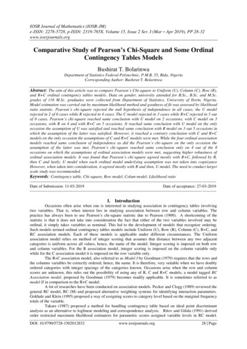
rather than odds are used in ordinal regression for the same reason as in logistic regression(i.e. they do not suffer from the ceiling and floor effects that odds do, you should rememberthis from Module 4).The key assumption in ordinal regression is that the effects of any explanatory variables areconsistent or proportional across the different thresholds, hence this is usually termed theassumption of proportional odds (SPSS calls this the assumption of parallel lines but it‟s thesame thing). This assumes that the explanatory variables have the same effect on the oddsregardless of the threshold. For example if a set of separate binary logistic regressions werefitted to the data, a common odds ratio for an explanatory variable would be observed acrossall the regressions. In ordinal regression there will be separate intercept terms at eachthreshold, but a single odds ratio (OR) for the effect of each explanatory variable. This is bestexplained by an example.As example using gender and English NC levelAs a simple example let‟s start by just considering gender as an explanatory variable. Beforeyou start building your model you should always examine your „raw‟ data. Figure 5.3.2 showsthe cross tabulation of English level by gender.Figure 5.3.2: Gender by English level crosstabulationClearly girls tend to achieve higher outcome levels in English than boys. What does this looklike in terms of the cumulative proportions and cumulative odds? In Figure 5.3.3 we calculatethe cumulative odds separately for boys and for girls.
Figure 5.3.3: Cumulative odds for English NC level separately for boys and girlsBoysCumulative N boysCumulative proportionCumulative oddsCumulative 620030.280.39-0.9575030.070.08-2.59GirlsCumulative N girlsCumulative proportionCumulative oddsCumulative 1628410.410.69-0.3878260.120.13-2.01Odds Ratio (Girls/Boys)Odds Ratio (Boys/Girls)-2.200.451.990.501.770.561.780.56We can calculate odds ratios by dividing the odds for girls by the odds for boys. In general theodds for girls are always higher than the odds for boys, as proportionately more girls achievethe higher levels than do boys. These odds ratios do vary slightly at the different categorythresholds, but if these ratios do not differ significantly then we can summarise therelationship between gender and English level in a single odds ratio and therefore justify theuse of an ordinal (proportional odds) regression. If we do calculate the odds ratio from anordinal regression model (as we will do below) this gives us an OR of 0.53 (boys/girls) orequivalently 1.88 (girls/boys), which is not far from the average across the four thresholds.This assumes the odds for girls of achieving level 4 are 1.88 greater than the odds for boys;the odds of girls achieving level 5 are 1.88 times greater than the odds for boys, and so onfor level 6 and level 7. i.e. that the odds of success for girls are almost twice the odds ofsuccess for boys, wherever you split the cumulative distribution (that is to say, whateverthreshold you are considering). SPSS has a statistical test to evaluate the plausibility of thisassumption, which we discuss on the next page (Page 5.4).
5.4 Running an ordinal regression on SPSSSo let‟s see how to complete an ordinal regression in SPSS, using our example of NC Englishlevels as the outcome and looking at gender as an explanatory variable.Data preparationBefore we get started, a couple of quick notes on how the SPSS ordinal regression procedureworks with the data, because it differs from logistic regression. First, for the dependent(outcome) variable, SPSS actually models the probability of achieving each level or below(rather than each level or above). This differs from our example above and what we do forlogistic regression. However this makes little practical difference to the calculation, we justhave to be careful how we interpret the direction of the resulting coefficients for ourexplanatory variables. Don‟t worry; this will be clear in the example. Second, for categorical(nominal or ordinal) explanatory variables, unlike logistic regression, we do not have theoption to directly specify the reference category (LAST or FIRST, see Page 4.11) as SPSSordinal automatically takes the LAST category as the reference category. So for our gendervariable (scored boys 0, girls 1) girls will be the reference category and the coefficients willbe for boys. Again this is not a huge problem because if we want to we can simply RECODEour variables to force a particular category as the reference category (e.g. if we wanted boysto be the reference category we could recode gender so girls 0 and boys 1). It is, however,slightly fiddly and annoying!Requesting an ordinal regressionYou access the menu via: Analyses Regression Ordinal. The window shown belowopens. Move English level (k3en) to the „Dependent‟ box and gender to the „Factor(s)‟ box.
Next click on the „Output‟ button. Here we can specify additional outputs. Place a tick in CellInformation. For relatively simple models with a few factors this can help in evaluating themodel. However, this is not recommended for models with many factors or for models withcontinuous covariates, since such models typically result in very large tables which are oftenof limited value in evaluating the model because they are so extensive (they are so extensive,in fact, that they are likely to cause severe mental distress). Also place a tick in the Test ofparallel lines box. This is essential as it will ask SPSS to perform a test of the proportionalodds (or parallel lines) assumption underlying the ordinal model (see Page 5.3).You also see here options to save new variables (see under the „Saved Variables‟ heading)back to your SPSS data file. This can be particularly useful during model diagnostics. Put atick in the Estimated response probabilities box. This will save, for each case in the data file,the predicted probability of achieving each outcome category, in this case the estimatedprobabilities of the student achieving each of the levels (3, 4, 5, 6 and 7).That is all we need to change in this example so click Continue to close the submenu andthen OK on the main menu to run the analysis.Examining the SPSS ordinal outputSeveral tables of thrilling numeric output will pour forth in to the output window. Let‟s workthrough it together. Figure 5.4.1 shows the Case processing summary. SPSS clearly labelsthe variables and their values for the variables included in the analysis. This is important tocheck you are analysing the variables you want to. Here I can see we are modelling KS3English level in relation to gender (with girls coded 1).
Figure 5.4.1: Case Processing SummaryFigure 5.4.2 shows the Model fitting information. Before we start looking at the effects of eachexplanatory variable in the model, we need to determine whether the model improves ourability to predict the outcome. We do this by comparing a model without any explanatoryvariables (the baseline or „Intercept Only‟ model) against the model with all the explanatoryvariables (the „Final‟ model - this would normally have several explanatory variables but at themoment it just contains gender). We compare the final model against the baseline to seewhether it has significantly improved the fit to the data. The Model fitting Information tablegives the -2 log-likelihood (-2LL, see Page 4.6) values for the baseline and the final model,and SPSS performs a chi-square to test the difference between the -2LL for the two models.Figure 5.4.2: Model FitThe significant chi-square statistic (p .0005) indicates that the Final model gives a significantimprovement over the baseline intercept-only model. This tells you that the model gives betterpredictions than if you just guessed based on the marginal probabilities for the outcomecategories.The next table in the output is the Goodness-of-Fit table (Figure 5.4.3). This table containsPearson's chi-square statistic for the model (as well as another chi-square statistic based onthe deviance). These statistics are intended to test whether the observed data are consistentwith the fitted model. We start from the null hypothesis that the fit is good. If we do not rejectthis hypothesis (i.e. if the p value is large), then you conclude that the data and the modelpredictions are similar and that you have a good model. However if you reject the assumption
of a good fit, conventionally if p .05, then the model does not fit the data well. The results forour analysis suggest the model does not fit very well (p .004).Figure 5.4.3: Goodness of fit testWe need to take care not to be too dogmatic in our application of the p .05 rule. For examplethe chi-square is highly likely to be significant when your sample size is large, as it certainly iswith our LSYPE sample of roughly 15,000 cases. In such circumstances we may want to set alower p-value for rejecting the assumption of a good fit, maybe p .01. More importantly,although the chi-square can be very useful for models with a small number of categoricalexplanatory variables, they are very sensitive to empty cells. When estimating models with alarge number of categorical (nominal or ordinal) predictors or with continuous covariates,there are often many empty cells (as we shall see later). You shouldn't rely on these teststatistics with such models. Other methods of indexing the goodness of fit, such as measuresof association, like the pseudo R2, are advised.In linear regression, R2 (the coefficient of determination) summarizes the proportion ofvariance in the outcome that can be accounted for by the explanatory variables, with larger R2values indicating that more of the variation in the outcome can be explained up to a maximumof 1 (see Module 2 and Module 3). For logistic and ordinal regression models it not possibleto compute the same R2 statistic as in linear regression so three approximations are computedinstead (see Figure 5.4.4). You will remember these from Module 4 as they are the same asthose calculated for logistic regression.Figure 5.4.4: Pseudo R-square StatisticsWhat constitutes a “good” R2 value depends upon the nature of the outcome and theexplanatory variables. Here, the pseudo R2 values (e.g. Nagelkerke 3.1%) indicates thatgender explains a relatively small proportion of the variation between students in theirattainment. This is just as we would expect because there are numerous student, family andschool characteristics that impact on student attainment, many of which will be much moreimportant predictors of attainment than any simple association with gender. The low R2indicates that a model containing only gender is likely to be a poor predictor of the outcome
for any particular individual student. Note though that this does not negate the fact that thereis a statistically significant and relatively large difference in the average English level achievedby girls and boys.The Parameter estimates table (Figure 5.4.5) is the core of the output, telling us specificallyabout the relationship between our explanatory variables and the outcome.Figure 5.4.5: Parameter Estimates TableThe threshold coefficients are not usually interpreted individually. They just represent theintercepts, specifically the point (in terms of a logit) where students might be predicted into thehigher categories. The labelling may seem strange, but remember the odds of being level 6 orbelow (k3en 6) is just the complement of the odds of being level 7; the odds of being level 5or below (k3en 5) are just the complement of the odds of being level 6 or above, and so on.While you do not usually have to interpret these threshold parameters directly we will explainbelow what is happening here so you understand how the model works. The results of ourcalculations are shown in Figure 5.4.6.Let‟s start with girls. Since girls represent our base or reference category the cumulative logitsfor girls are simply the threshold coefficients printed in the SPSS output (k3en 3, 4, 5, 6).We take the exponential of the logits to give the cumulative odds (co) for girls. Note that thesedo not match the cumulative logits and odds we showed in Figure 5.3.3 because, asexplained above, SPSS creates these as the odds for achieving each level or below asopposed to each level or above and because the reference category is boys not girls.However once these logits are converted to cumulative proportions/probabilities you can seethey are broadly equivalent in the two tables (bar some small differences arising from theassumption of proportional odds in the ordinal model, more on which later). We calculate thepredicted cumulative probabilities from the cumulative odds (co) simply by the formula1/(1 co). If we want to find the predicted probability of being in a specific outcome category(e.g., at a specific English level) we can work out the category probability by subtraction. So ifthe probability of being at level 7 is 0.12 (or 12%), and the probability of being at level 6 or
above is 0.41 (or 41%), then the probability of being specifically at level 6 is .41 - .12 .29 (or29%). Similarly the predicted probability for being specifically at Level 5 for girls is .80 - .41 .39 (39%) and at level 4 it is .93 - .80 .13 (13%). Finally the probability of being at level 3 is 1- .93 .07 (7%).Figure 5.4.6: Parameters from the ordinal regression of gender on English level.BoysCumulative logitCumulative odds [exp(Cum.logit )]Cumulative proportion [1/(1 exp(Cum.logit )]Category probability31.000.13English mulative logitCumulative odds [exp(Cum.logit )]Cumulative proportion [1/(1 exp(Cum.logit )]Category 0.800.3960.3541.420.410.2971.9887.300.120.12Odds Ratio (Girls/Boys)Odds Ratio 32.670.270.2072.61713.690.070.07To calculate the figures for boys (gender 0) we have to combine the parameters for thethresholds with the gender parameter (-.629, see Figure 5.4.5). Usually in regression we addthe coefficient for our explanatory variable to the intercept to obtain the predicted outcome(e.g. y a bx, see modules 2 & 3). However in SPSS ordinal regression the model isparameterised as y a - bx. This doesn‟t make any difference to the predicted values, but isdone so that positive coefficients tell you that higher values of the explanatory variable areassociated with higher outcomes, while negative coefficients tell you that higher values of theexplanatory variable are associated with lower outcomes. So for example the cumulative logitfor boys at „level 4 ‟ is -2.543 - (-.629) -1.914, at level 5 it is -1.376 - (-.629) -.747 and soon. Then, just as for girls, the cumulative odds (co) are the exponent of the logits, thecumulative proportions are calculated as 1/(1 co), and the category probabilities are found bysubtraction in the same way as described for girls. Phew!Odds RatiosWe can divide the odds for girls by the odds for boys at each cumulative split to give the OR(see Figure 5.4.6). We can see that in the proportional odds model the OR is constant (0.53)at all cumulative splits in the data (the odds of boys achieving a higher level are approximatelyhalf the odds for girls). We can express the OR the other way round by dividing the odds for
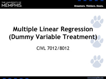
boys by the odds for girls which gives us the OR of 1.88 (the odds for girls of achieving ahigher level are approximately twice the odds for boys). As we saw in Module 4 these OR of0.53 and 1.88 are equivalent, they just vary depending on the reference category. (seeExtension D - you can convert an OR to its complement by dividing the OR into 1, e.g.1/0.53 1.88, equally 1/1.88 0.53). The important thing to note here is that the gender OR isconsistent at each of the cumulative splits in the distribution.The above was completed just to demonstrate the proportional odds principle underlying theordinal model. In fact we do not have to directly calculate the ORs at each threshold as theyare summarised in the parameter for gender. This shows the estimated coefficient for genderis -.629 and we take the exponent of this to find the OR with girls as the base: exp(-.629) 0.53. To find the complementary OR with boys as the base just reverse the sign of thecoefficient before taking the exponent, exp(.629) 1.88. The interpretation of these ORs is asstated above.Test of parallel linesRemember that the OR is equal at each threshold because the ordinal model has constrainedit to be so through the proportional odds (PO) assumption. We can evaluate theappropriateness of this assumption through the „test of parallel lines‟. This test compares theordinal model which has one set of coefficients for all thresholds (labelled Null Hypothesis), toa model with a separate set of coefficients for each threshold (labelled General). If thegeneral model gives a significantly better fit to the data than the ordinal (proportional odds)model (i.e. if p .05) then we are led to reject the assumption of proportional odds. This is theconclusion we would draw for our example (see Figure 5.5.7), given the significant value asshown below (p .004).Figure 5.4.7: Test of Parallel LinesNote: The sharp-eyed among you may have noted that the chi-square statistics given above for theTest of Parallel Lines is exactly the same as that given for the omnibus test of the ‘goodness of fit’ ofthe whole model. This is because we have only a single explanatory variable in our model, so the twotests are the same. However when we have multiple explanatory variables this will not be the case.We can see why this is the case if we compare our OR from the ordinal regression to theseparate ORs calculated at each threshold in Figure 5.3.3. While the odds for boys areconsistently lower than the odds for girls, the OR from the ordinal regression (0.53)underestimates the extent of the gender gap at the very lowest level (Level 4 OR 0.45) and
slightly overestimates the actual gap at the highest level (level 7 OR .56). We see how thisresults in the significant chi-square statistic in the „test for parallel lines‟ if we compare the„observed‟ and „expected‟ values in the „cell information‟ table you requested, shown below asFigure 5.4.8. The use of the single OR in the ordinal model leads to predicting fewer boys andmore girls at level 3 than is actually the case (shown by comparing the „expected‟ numbersfrom the model against the „observed‟ numbers).Figure 5.4.8: Output for Cell InformationHowever the test of the proportional odds assumption has been described as anticonservative, that is it nearly always results in rejection of the proportional odds assumption(O‟Connell, 2006, p.29) particularly when the number of explanatory variables is large (Brant,1990), the sample size is large (Allison, 1999; Clogg & Shihadeh, 1994) or there is acontinuous explanatory variable in the model (Allison, 1999). It is advisable to examine thedata using a set of separate logistic regression equations to explicitly see how the OR
5.4 Example 1 - Running an ordinal regression on SPSS 5.5 Teacher expectations and tiering 5.6 Example 2 - Running an ordinal regression for mathematics tier of entry 5.7 Example 3 - Evaluating in