WIXLIB

Spectral Analysis in RHelen J. WearingJune 8, 2010Contents1 Motivation12 What is spectral analysis?23 Assessing periodicity of model output74 Assessing periodicity of real data115 Other details and extensions121MotivationCyclic dynamics are the rule rather than the exception in infectious disease data, which may be dueto external forcing by environmental drivers or the inherent periodicity of immunizing (or partiallyimmunizing) infections or a combination of both. As an example, plotted in the figure below are weeklycase reports of childhood diseases from Copenhagen, Denmark during the mid-twentieth century.1

0200 400 600 1940195019601940Date.219501960Date.3What types of questions might we ask of these data? In this module, we introduce how to estimate theperiodicity of time series using spectral analysis. Specifically, we will look at recurrent epidemics fromeither simulated or real data. We can often use these summary metrics as probes to match model outputto data.2What is spectral analysis?In a nutshell: the decomposition of a time series into underlying sine and cosine functions of differentfrequencies, which allows us to determine those frequencies that appear particularly strong or important.Let’s briefly re-familiarize ourselves with sine and cosine functions!2

1.00.0 1.0 0.5x0.5cos(4 pi t)sin(4 pi t) 1.0 0.50.00.51.0tThe frequency (f ) of a sine or cosine function is typically expressed in terms of the number of cyclesper unit time. For example, in the above figure the frequency of each function is 2 cycles per unit time.The period (T ) of a sine or cosine function is defined as the length of time required for one full cycle.Thus, it is the reciprocal of the frequency (T 1/f ). In the above figure T 1/2.Fitting sine wavesOne way of viewing spectral analysis is as a linear multiple regression problem, where the dependentvariable is the observed time series, and the independent variables are the sine functions of all possible(discrete) frequencies.Suppose we have a time series xt of length n, for convenience assume n is even. We can fit a time seriesregression with xt as the response and the following n 1 predictor variables: 2πt2πt2(n/2 1)πt2(n/2 1)πtcos, sin, . . . , cos, sin, cos(πt)nnnnIf we represent the estimated regression coefficients by a1 , b1 , . . . , an/2 1 , bn/2 1 , an/2 , respectively, wecan write xt asn/2 1Xxt a 0 [ak cos(2πkt/n) bk sin(2πkt/n)] an/2 cos(πt)(1)k 13

The cosine parameters, ak , and sine parameters, bk , tell us the degree to which the respective functionsare correlated with the data. This regression model is a finite Fourier series for a discrete time series.Note that because the number of coefficients equals the length of the time series, there are no degreesof freedom for error. The intercept term, a0 , is just the mean, x̄, of the time series. The lowest possiblefrequency is one cycle, or 2π radians, per record length (which is 2π/n radians per sampling interval).A general frequency, in this representation, is k cycles per record length (2πk/n radians per samplinginterval). The highest frequency is 0.5 cycles per sampling interval (π radians per sampling interval).We should pay close attention to the sampling interval and record length. Many time series are ofa variable that is continuous in time but is sampled to give a time series at discrete time steps. Thesampling interval (or sampling rate) constrains the highest frequency (known as the Nyquist frequency)that we can detect. For example, if we sample every week, we cannot detect cycles less than 2 weeks inlength. On the other hand, the length of the time series determines the lowest frequency that we candistinguish.PeriodogramThe periodogram quantifies the contributions of the individual frequencies to the time series regressionand is defined asPk a2k b2kwhere Pk is the periodogram value at frequency k (for k 1, . . . , n/2). The periodogram values canbe interpreted in terms of variance of the data at the respective frequency or period. A plot of Pk , asspikes, against k is a Fourier line spectrum. The raw periodogram in R is obtained by joining the tips ofthe spikes in the Fourier line spectrum to give a continuous plot and scaling it so that the area equalsthe variance.Although we have introduced the periodogram in the context of a linear multiple regression, the calculations are usually performed with the fast Fourier transform algorithm (FFT) (and this is what R usestoo).To summarize, spectral analysis will identify the correlation of sine and cosine functions of differentfrequency with the observed data. If a large correlation (sine or cosine coefficient) is identified, you canconclude that there is a strong periodicity of the respective frequency (or period) in the data.Let’s consider a simple example to clarify the underlying ”mechanics” of spectrum analysis in R beforewe discuss further details of the technique.Simple ExampleWe will create a simple time series, and then see how we can extract the frequency information usingspectral analysis. First, create a time variable t and then specify the time-dependent variable x: t - seq(0,200,by 0.1) x - cos(2*pi*t/16) 0.75*sin(2*pi*t/5)The variable x is made up of two underlying periodicities: the first at a frequency of 1/16 or period of16 (one observation completes 1/16’th of a full cycle, and a full cycle is completed every 16 observations)and the second at a frequency of 1/5 (or period of 5). The cosine coefficient (1.0) is larger than the sinecoefficient (0.75).4

0.0 1.5x1.5 par(mfrow c(2,1)) plot(t,x,'l') spectrum(x)050100150200t1e 031e 18spectrumSeries: xRaw Periodogram0.00.10.20.30.40.5frequencybandwidth 0.000143The R command spectrum calculates the periodogram and automatically plots it against frequency.There are three technical points we should briefly discuss (and some we won’t but feel free to ask furtherquestions if you have any): pre-processing of the data smoothing of the periodogram how to make R output better looking and give more intuitive estimates of the spectral density!Preparing the Data for AnalysisUsually, we want to subtract the mean from the time series. Otherwise the periodogram and densityspectrum will mostly be ”overwhelmed” by a very large value for the first cosine coefficient (a0 ). In R, the spectrum function goes further and automatically removes a linear trend from the series beforecalculating the periodogram. It seems appropriate to fit a trend and remove it if the existence of a trend5

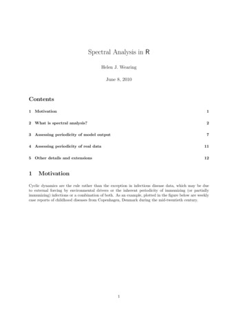
in the underlying stochastic process is plausible. Although this will often be the case, there may be casesin which you prefer not to remove a fitted trend and this can be accomplished using spec.pgram, whichgives the user more control over certain arguments.SmoothingThe periodogram distributes the variance over frequency, but it has two drawbacks. The first is that theprecise set of frequencies is arbitrary, in as much as it depends on the record length. The second is thatthe periodogram does not become smoother as the length of the time series increases but just includesmore spikes packed closer together. The remedy is to smooth the periodogram, and one way to do thisis by using a smoothing kernel of spikes before joining the tips. The smoothed periodogram is alsoknown as the sample spectrum. However, the smoothing will reduce the heights of peaks, and excessivesmoothing will blur the features we are looking for. It is a good idea to consider spectra with differentamounts of smoothing, and this is made easy for us with the R function spectrum. The argument spanis the number of spikes in the kernel. An alternative method for computing a smoothed spectrum is tocalculate the Fourier line spectrum for a number of shorter sub-series of the time series and average theline spectra of the subseries.Spectral analysis in RThe spectrum function defaults to a logarithmic scale for the spectrum, but we can change this bysetting the log parameter to ”no”. The default frequency axis is in cycles per sampling interval. It ismore intuitive to convert the frequency axis to cycles per unit time, we can do this by extracting thefrequency values that R returns and dividing by the length of the sampling interval. We should alsomultiply the spectral density by 2 so that the area under the periodogram actually equals the varianceof the time series. del -0.1 # sampling intervalx.spec - spectrum(x,log "no",span 10,plot FALSE)spx - x.spec freq/delspy - 2*x.spec specplot(spy spx,xlab "frequency",ylab "spectral density",type "l")6

100806040020spectral density012345frequency3Assessing periodicity of model outputLet’s now look at how all this works on simulated data. We will start by simulating the seasonal SIRmodel that was introduced yesterday. First, specify the model require(deSolve) seasonal.sir.model - function (t, x, params) { with( as.list(c(x,params)), { beta - beta0*(1 beta1*cos(2*pi*t)) dS - mu*(N-S)-beta*S*I/N dI - beta*S*I/N-(mu gamma)*I dR - gamma*I-mu*R res - c(dS,dI,dR) list(res) } ) }7

Then we simulate the model using lsoda and calculate the periodogram on the last part of the timeseries (after discarding transients).0.006times - seq(0,100,by 1/120)params - c(mu 1/50,N 1,beta0 1000,beta1 0.4,gamma 365/13)xstart - c(S 0.06,I 0.001,R 0.939)out - l,params,rtol 1e-12,hmax 1/120))par(mfrow c(3,1))plot(I time,data out,type 'l',subset time 40)Iend -subset(out,time 40,select c(I))del -1/120x.spec - spectrum(Iend,span 5,log "no",plot FALSE)spx - x.spec freq/delspy - 2*x.spec specplot(spy spx,xlab "frequency",ylab "smoothed spectral density",type "l")plot (spy spx, subset spx 2,xlab "frequency",ylab "spectral density",type "l") #Zoom-in on low freqdom.freq spx[which.max(spy)] #Extract the dominant frequency0.000I 4050607080901004050600.00100.0000smoothed spectral densitytime01020300.00100.0000spectral densityfrequency0.00.51.01.52.0frequencyExercise 1. Explore the effects of changing amplitude of seasonality, β1 , on the periodicity of thismodel. Be careful to distinguish between transient and asymptotic dynamics. What happens if you logtransform the simulated data and then apply the spectrum?8

**Exercise 2. Construct a figure that illustrates the relationship between β1 and the dominant periodof the output.Stochastic modelAs you saw yesterday, the dynamics of the deterministic SIR model without seasonality are dampedoscillations toward an equilibrium. In the stochastic version, you probably saw a lot of extinction becausethe populations you looked at were small and there was no import parameter. Below is some code tosimulate the stochastic SIR model using the tau-leap method for a population of 1 million and witha small import parameter ν. What you find is that demographic stochasticity amplifies the intrinsicoscillations of the system and we observe sustained cycles.The tau-leap code describing the SIR model with births and deaths: sir.birth.death.onestep.tauleap - function (x, params) {S - x[2]I - x[3]R - x[4]N - S I Rwith(as.list(params),{births -min(S,rpois(1,mu*N*tau))Sdeaths -min(S,rpois(1,mu*S*tau))Ideaths -min(I,rpois(1,mu*I*tau))Rdeaths -min(R,rpois(1,mu*R*tau))dSI - min(S,rpois(1,beta*S*(I/N nu)* tau))dIR - min(I,rpois(1,gamma*I * tau))new.sir -cbind(S births-Sdeaths- dSI , I -Ideaths dSI - dIR, R -Rdeaths dIR)cbind(tau,new.sir)})}As before, we set parameters and loop through the process: sir.birth.death.model - function (x, params, nstep) { X - array(dim c(nstep 1,4)) colnames(X) - c("time","S","I","R") X[1,] - x for (k in 1:nstep) { X[k 1,] - x - sir.birth.death.onestep.tauleap(x,params) } X }Now let’s simulate and plot the resulting time series: set.seed(38499583) nsims - 1 pop.size - 10000009