Transcription
Precision Jitter AnalysisUsing theAgilent 86100C DCA-JProduct Note 86100C-1
IntroductionThe extremely wide bandwidth of equivalent-timesampling oscilloscopes makes them the tool of choicefor precision analysis of very high-speed waveforms.Historically, low sampling rates have limited their abilityto perform in-depth jitter analysis. A revolutionary newsampling/acquisition system in the Agilent 86100C hastransformed the sampling oscilloscope into a precisionjitter analysis tool. Complete jitter characterization isavailable including: Jitter analysis from 50 Mb/s to over 40 Gb/s Extremely high sensitivity through lowintrinsic jitter (“jitter noise floor”, as low as200 femtoseconds) Very simple setup and measurements, typicallyachieved with a single button press Separation into random and severaldeterministic jitter classes Both histogram and tabular displays of alljitter elements Jitter analysis linked with precision waveformdisplays for deeper insight into signal behaviorThis product note will review the new jitter measurementcapabilities of the 86100C as well as the architecturalchanges (both hardware and algorithmic) that enablethem. A review of the jitter measurement procedureswill be presented to allow users to quickly get accurateresults. The measurement results will then be reviewedand interpreted. Frequently asked questions andanswers are presented.The jitter measurement approach is new and hencea very detailed analysis is provided describing thetechnique. However, the process of performing ajitter measurement is extremely simple and in mostcases can be performed in a single button press.To begin making jitter measurements immediately,go directly to page 13.Jitter measurements require an 86100C mainframewith option 001 hardware and option 100 jitteranalysis software.2
Table of ContentsIntroduction . . . . . . . . . . . . . . . . . . . . . . . . . . . . . . . . . . 2Table of Contents . . . . . . . . . . . . . . . . . . . . . . . . . . . . . . 3Jitter Analysis Using the Agilent 86100C DCA-J . . . . . . 4The Case for Jitter Separation . . . . . . . . . . . . . . . . . . . . 4The 3 Gb/s Measurement Barrier . . . . . . . . . . . . . . . . . . 6Historical Limitations of Legacy SamplingOscilloscopes for Jitter Analysis . . . . . . . . . . . . . . . . . 6Architectural changes yield fast andaccurate measurements . . . . . . . . . . . . . . . . . . . . 8Deriving a pattern trigger withinthe oscilloscope . . . . . . . . . . . . . . . . . . . . . . . . . . 8Increasing measurement speed throughoptimized sampling . . . . . . . . . . . . . . . . . . . . . . . 9Using the New Architecture to Separate Jitter . . . . . . 10Correlated jitter . . . . . . . . . . . . . . . . . . . . . . . . . . . 10Uncorrelated jitter . . . . . . . . . . . . . . . . . . . . . . . . . 11Aggregate deterministic jitter (DJ) . . . . . . . . . . . . 12Aggregate total jitter (TJ) . . . . . . . . . . . . . . . . . . . 12Basic Procedure For Making JitterMeasurements With the 86100C DCA-J . . . . . . . . . . 13Interpreting Measurement Results . . . . . . . . . . . . . . . . 20MJSQ: Fibre Channel – Methodologies forJitter and Signal Quality Specification . . . . . . . . . . . 21Understanding the Accuracy of Jitter MeasurementsPerformed with the 86100C DCA-J . . . . . . . . . . . . . 22Frequently Asked Questions (FAQ’s) . . . . . . . . . . . . . . 243
Jitter Analysis Using the Agilent 86100C DCA-JThe Case for Jitter SeparationVirtually every high-speed communications designmust deal with the issue of jitter. Definitions of jitteras well as its impact on system performance have beenwell documented but can be generally summarized asfollows: When data are misplaced from their expectedpositions in time, receiver circuits can make mistakesin trying to interpret logic levels. Bit error ratio (BER)is degraded.In many communications systems and standards,specifying jitter involves determining how much jittercan be on transmitted signals. Jitter is analyzed fromthe approach that for a system to operate with very lowBER’s (1 error per trillion bits being common), it must beaccurately characterized at corresponding levels ofprecision. This is facilitated through separating theunderlying mechanisms of jitter into classes thatrepresent root causes. Specifically, jitter is brokenapart into its random and deterministic components.The deterministic elements are further broken downinto a variety of subclasses. With the constituentelements of jitter identified and quantified, the impactof jitter on BER is more clearly understood. This thenleads to straightforward system budget allocations andsubsequent device/component specifications.As data rates increase, jitter problems tend to bemagnified. What might have been considered a smalland tolerable time deviation at a lower data rateappears to be large and intolerable at high data rates.Consider that the bit period of a 10 Gb/s signal isonly 100 picoseconds. When combined with signalimpairments such as attenuation, dispersion, andnoise, just a few picoseconds of timing instabilitycan mean the difference between achieving or failingto reach BER objectives. The problem is furtheraggravated by the difficulty presented in makingaccurate measurements of jitter. A variety ofmeasurement approaches exist. While the variousmethods are well thought out and are based uponsound architectures, there has been frustration withinthe industry around the complexity of setting up ameasurement, getting repeatable results, and perhapsmore important, getting the various techniques toagree with each other. The measurement problemis severely compounded when the 3 Gb/s data ratethreshold is crossed. Above this rate, the list ofsolutions for jitter measurements is short. The“equivalent time” sampling oscilloscope, withconfigurations having over 80 GHz of bandwidth andextremely low levels of intrinsic jitter, is an obviouscandidate for jitter measurements at very high datarates. However, some fundamental limitations ofthe wide-bandwidth oscilloscope have historicallyprevented it from being more than just a coarse jittermeasurement tool. These limitations have now beenovercome with the new Agilent 86100C DCA-J.Patented architectural changes have resulted in aflexible and easy to use jitter solution based upon afamiliar laboratory instrument. Perhaps most importantis that this tool provides thorough and accurate jitteranalysis at rates from 50 Mb/s to over 40 Gb/s. Thecombination of highly accurate jitter analysis withthe most accurate oscilloscope make this an essentialtool for any high-speed digital communicationstest system.4Breaking jitter into its constituent elements allows aprecision measurement of the total jitter on a signal, evento extremely low probabilities. In addition to accuracy,the extensive measurement times often required toassess rare phenomenon can be dramatically reduced.To understand the approach, it is helpful to reviewthe various types of jitter that can exist on a signal.The first classification is between jitter that is randomand that which is not. Jitter that is not random isbounded. That is, its magnitude is finite. In contrast,random jitter is unbounded and within physical limits,can theoretically reach any magnitude. Random jitter(RJ) is often described as having a Gaussian distributionwith ‘tails’ that extend indefinitely. Random jittermechanisms are often due to oscillator phase noise, wherethe clock used to set data rates cannot produce a purefrequency and exhibits a random deviation from the ideal.Deterministic jitter (DJ) can be broken into severalsubclasses. The first division is between that whichis correlated to the data sequence or pattern and thatwhich occurs independent of the data. This can bereferred to as correlated and uncorrelated DJ. (Notethat RJ is also a class of uncorrelated jitter, but isunbounded and not deterministic).Uncorrelated DJ is most often observed as some formof periodic phase modulation of clocks used to setdata rates. This DJ is uncorrelated because itsmagnitude is independent of where it is observed inthe pattern. Because this jitter is periodic, it is oftenreferred to as periodic jitter or PJ. Uncorrelated jittercan also be due to bounded, but non-periodic sources.Any one-time transient event that causes edgemisplacement would be a non-periodic uncorrelatedjitter. Its effects would be bounded. This type of jitteris likely not observed, except by coincidence, unlessthe measurement system were synchronized to themechanism in some way. For a sampling scopemeasurement system, this type of jitter would haveto systematically repeat to be observed, and wouldthen in effect become a periodic jitter element.
Jitter that is correlated to the data pattern can bebroken into three categories: Inter-symbol interference(ISI), duty-cycle distortion (DCD), and subrate jitter(SRJ). Measurement of these jitter sources requireseach edge in the data pattern be observed.In that ISI and DCD are pattern dependent, they arepart of a jitter class called data dependent jitter or DDJ.SRJ jitter can be viewed as a form of uncorrelated PJor a form of DDJ, depending upon how it is manifestedin the data pattern. Consider a multiplexing schemewhere one leg of a data serializer is physically longerthan intended. Any bit on this leg is possibly retardedcompared to others on different legs. See page 10 formore details on subrate jitter measurements andinterpretation.ISI mechanisms are well known for their impact ondigital communications. Reduced or insufficientbandwidth results in reduced edgespeeds. Thus as atransition takes place from a 1 to a 0 or a 0 to a 1, thesignal may not reach its intended amplitude beforeit is required to switch logic levels again. Obviouslythis will result in vertical eye closure. However,this will also result in both retarded and advancededges relative to their ideal positions. The level ofmisplacement is typically a function of the data patternpreceding the edge being observed. (An example ofthis is discussed on pages 16–19.)It is important to reiterate what can be achievedwhen the various components of jitter can be isolated.Obviously it helps in troubleshooting jitter problems,as the nature/type of the jitter is often a key indicatorof the source. A less obvious reason is that it providesa method to accurately assess the aggregate jittermagnitude to very low probabilities without the timerequired for a direct measurement. The key to theapproach is to be able to segregate the RJ from allother sources. This allows a precision assessmentof the distribution of the jitter. The extreme jittermagnitudes are effectively the low probability tailsdue to RJ. Thus determining these values is achievedonce the RJ standard deviation is known, in additionto knowing how the deterministic elements interactwith the RJ. This is discussed in the remainder ofthe paper.DCD is observed when the durations of logic 1 pulsesare different than the duration of logic 0 pulses. It iseasily observed in the eye diagram as the nominal eyecrossing (where rising edges intersect falling edges)occurring somewhere other than the 50% amplitudepoint. In that jitter is typically characterized at the 50%amplitude level, rising and falling edges intersectingat a level other than the 50% amplitude implies thatedges are misplaced from their ideal positions.ISIDDJDCDDJSRJTJPJRJFigure 1. Total jitter is composed of several types of jitter5
The 3 Gb/s Measurement BarrierThere are a number of well-established tools for jitteranalysis. For most, the hardware used to acquireinformation allows measurements at data rates up to3 Gb/s and slightly beyond. Thus as systems are beingdeveloped requiring transmission rates of 4, 6, and 10Gb/s, different measurement technologies are required.The wide-bandwidth oscilloscope has a bandwidth inexcess of 80 GHz, thus these instruments’ operatingranges are more than sufficient for general waveformanalysis to 40 Gb/s and beyond. For the wide-bandwidthoscilloscope, rates that can be measured are dependenton channel bandwidth. Typically, the bandwidth shouldbe at least double the data rate, with bandwidthsranging from 20 to 50, 70 and 80 GHz dependingupon the oscilloscope plug-in configuration. As theoscilloscope is DC coupled, low data rates are alsowithin its measurement range.Historical Limitations of Legacy SamplingOscilloscopes for Jitter AnalysisWhere does the wide-bandwidth sampling oscilloscopefit into the jitter analysis picture? At a first glance,this instrument looks very attractive due to its verylow jitter noise floor and the previously mentionedwide bandwidth. Historically, several barriers haveexisted for efficient and accurate measurementsof jitter. Fortunately, the Agilent 86100 DCA hasundergone significant architectural changes toovercome these issues. The new Agilent 86100C isreferred to as the DCA-J, indicating its functionalityas a digital communications analyzer with extensivejitter analysis capability.The three key historical limitations of equivalent timesampling oscilloscopes, when they are used for jitteranalysis are: Excessive measurement times due to a relativelyslow data acquisition rate Requirement of a pattern trigger Timing measurement errors introduced whenlarge ranges of timebase delay are usedWhile the bandwidth of these oscilloscopes is extremelyhigh, the rate at which data is obtained is relativelyslow, at well under 1 Msample/s. This is in contrastwith “real-time” oscilloscopes, that have bandwidths 10 GHz, but which acquire data at rates of upto 40 Gsamples/s. The sampling oscilloscope then hasspecial requirements for the data it can analyze. Thesignals must be repetitive, as it will take several passesto acquire enough samples to accurately reconstructa waveform. (An exception to the repetitive signalrequirement is the eye diagram. In this case, samplesare acquired at essentially random, but synchronouslocations in a bitstream. The common eye diagram isthen a composite of samples acquired throughout thestream of data.)The simplest jitter analysis performed on samplingoscilloscopes consists of projecting a pixel high sliceof the eye diagram at the crossing point along thetime axis (Fig. 2). This approximates the probabilitydistribution function of the signal’s jitter.6
Figure 2. Jitter observed through the histogram of the eye diagramcrossing pointThe crossing point histogram can be post-processedto provide rudimentary jitter analysis: RJ and DJ canbe separated by fitting Gaussian tails to the histogramand TJ can be extrapolated. However, because of thelow sampling rate and fluctuations in the histogrampopulation over time, this simple analysis tends tobe coarse.The sampling scope still has the potential to do anaccurate jitter measurement. The DDJ can be found byproviding a pattern or frame trigger to the oscilloscope.The pattern trigger provides a timing edge that occursat most once per repetition of the data pattern. Thus,a requirement for the DDJ measurement is a repeatingdata pattern. RJ, and DJ that is not correlated to thedata pattern can be eliminated from the measurementby enabling trace averaging. The location of eachedge can be compared to its ideal location throughcomparison to the clock edge position (if also displayedon the scope) or by comparison of its position relativeto the subsequent position measurement of all theother bits in the pattern.The RJ and uncorrelated PJ can be measured bydisabling any trace averaging and measuring a singledata edge in the pattern. (Thus the pattern triggerrequirement is still in place). Since all the samplesare acquired on a single edge, there will be no DDJcomponent in these data. A data slice at the edgemidpoint can be used to generate a time axis histogramthat will contain the RJ and uncorrelated PJ. Thehistogram can then be analyzed and fitted to a curveto determine the critical statistics of these two jitterelements.While this process is superior to a simple histogramof the eye crossing point in terms of precision andthe separating out of the jitter elements, it still hassome serious flaws. Perhaps the most important isthe amount of time required to acquire a sufficientpopulation for an accurate measurement. Considerthat an oscilloscope trace of a data edge is composedof perhaps 100 to 1000 samples. The time betweensamples is several microseconds (25 microsecondsfor the Agilent 86100). Thus it can take 25 millisecondsto produce one edge from which a single jitter valuecan be obtained. Several jitter values are requiredto obtain sufficient data to produce a significantpopulation from which the RJ and uncorrelated PJvalues might be obtained. The time required for thisanalysis can easily approach several minutes.The situation is more severe when attempting todetermine the DDJ, as each edge in the pattern mustbe analyzed. For an accurate measurement, only a fewedges are acquired for any section of the waveformpattern being examined rather than attemptingto measure a large number of edges at a reducedresolution. To remove the uncorrelated jitter elements,trace averaging is used. Thus the number of pointsthat must be acquired is multiplied by the averagingfactor, perhaps 16. While the time required for ashort pattern is manageable and might take a minuteor two, patterns such as a 215–1 PRBS (32767 bits)can take many hours to measure.A second problem with this sampling oscilloscopemethod is the requirement of a pattern trigger. Thatis, a trigger coincident with the repetition of thepattern (sometimes also called a frame trigger). Whilethis may be easy to obtain in a test system using aninstrumentation pattern generator, many test scenarioswill not have this signal readily available. Additionally,the pattern trigger from a pattern generator instrumentwill typically have some data dependent jitter associatedwith it. This can corrupt the measurement, particularlywhen measuring low levels of jitter.A third limitation associated with legacy equivalenttime sampling oscilloscope architectures is a time errorthat is introduced by using large ranges of timebasedelay (required to observe events that occur significantamounts of time after the reference trigger event). Intraditional applications of these oscilloscopes, thishas not typically been a problem. However, in orderto characterize jitter through a pattern (primarilyfor DDJ), large ranges of timebase delay are typicallyrequired. This can introduce significant error into thejitter measurement.Thus, long test times, the requirement of a patterntrigger, and measurement error from large rangesof timebase delay present significant obstacles for thesampling oscilloscope jitter solution.7
Architectural Changes Yield Fast and AccurateMeasurementsTo overcome these historical limitations, fundamentalchanges to the sampling oscilloscope architectureare required. Once the architecture is improved, thedoor opens for new measurement algorithms, which candramatically reduce the time required and significantlyimprove the accuracy for jitter measurements.Deriving a pattern trigger within the oscilloscopeA pattern trigger can be derived from a system clocksignal. One must know the length of the pattern andthe ratio of the data rate to the system clock rate. Forexample, in the case of the full rate clock, if the patternlength is N, a strobe signal should be generated everytime that N clock cycles have been counted. While theconcept is very simple, a successful implementation isfar from trivial. Consider that any timing imperfectionsor asynchronism in generating the trigger are manifesteddirectly in jitter measurement error. It is also importantfor the sampling oscilloscope to have control of thepattern trigger and where it fires in relationship to thepattern. This control enables the oscilloscope to targetthe sampling at specific locations in the data patternand to force the data acquisition to be performedover a small range of the timebase. Thus, the internallygenerated pattern trigger architecture has eliminatedboth the requirement for a pattern trigger as wellas measurement errors induced by large ranges oftimebase delay.With the internally generated and controlled patterntrigger, the oscilloscope can now systematically ‘walk’through the pattern and determine the nominal locationof each edge in the sequence. When executing thisfunction, averaging is used to remove any uncorrelatedjitter mechanisms in order to best determine theaverage location of each edge. The next significantchange in this new approach to jitter measurementrequires a method for dramatically increasing themeasurement speed.Clock in50 MHz to 13 GHzTriggerProgrammable divider(2, 4, 8, 16, 32)Re-timerHigh-speed counter(25 to 725 MHz)Figure 3: 86100C conceptual diagram for internally deriving a pattern trigger8Count Pulse23(1, 2, 3, ., 2 )
Increasing measurement speed throughoptimized samplingGiven that the sampling rates of equivalent timeoscilloscopes are slow, improving the speed of jittermeasurements requires that data be collected andprocessed in a fashion where as many samples aspossible contribute directly to the jitter measurement.The main candidate for improvement stems from thefact that, historically, a single jitter value is derivedfrom hundreds of waveform samples. This is because theoscilloscope is fundamentally an amplitude measuringinstrument. To determine the position of an edge, manysamples were required to reconstruct the waveform edge,and from that only a single jitter value was derived.To improve the jitter measurement efficiency of theoscilloscope, two important changes are made to howsamples are collected. First, rather than collectingsamples from all portions of the waveform includingwhere amplitude is somewhat constant (and hence thereis no direct jitter information), samples are acquiredonly from edges. However, this alone would not solvethe problem, as many amplitude samples from theedge would still be required to yield a single edge timeposition and thus a single jitter measurement data point.The key enabler to measurement efficiency is to developa transfer function that allows the amplitude of anysingle sample taken from an edge to be directly translatedto a jitter measurement value. This is achieved bygenerating models of the edges.Consider the edge of figure 4. If the time of the samplingis set up to take place at the 50% amplitude or middleof the ideal, jitter free edge (this is enabled by theinternally generated and controlled pattern trigger), anearly arriving signal will have an amplitude above themiddle, while a late arriving edge will have an amplitudebelow the middle level. To determine the amount of jitteron the edge from which the sample was taken, one mustknow the amplitude versus time shape of the edge. Thisis effectively an amplitude-to-jitter transfer function an edge model. Once the edge is modeled, every samplethat is taken along the edge yields a jitter measurement.Two types of edge models are presented - single-edgemodels and composite-edge models. (The single edgemodels are used in uncorrelated jitter measurementswhile the composite edge models are used for datadependent jitter measurements. This is discussedlater). A single-edge model is constructed by taking1024 samples across the entire span of one edge.A mathematical function is constructed that deliversthe best fit, in a least squares sense, to the sampleddata. A composite-edge model is very similar, exceptthe samples used to construct the model are takenfrom multiple edges.A single-edge model is used to describe the amplitudeto-jitter characteristics of a specific edge of a pattern.Composite-edge models are composed of 4096 pointsand are used to describe the amplitude-to-jittercharacteristics of a class of edges. The shape of anedge can be dependent upon the preceding bits. The‘memory’ generally lasts for three or four bits, thusthere are several classes or groups of edge shapespossible. A class is defined by two factors - risingversus falling and the preceding bits. For example,‘00001’ is one class of rising edge, and ‘00101’ isanother. Similarly, ‘11110’ is one class of falling edge,and ‘11010’ is another. Consequently, 16 edge classesare defined – 8 rising and 8 falling.There is some measurement time overhead associatedwith generating edge models for the several edgeclasses. However, consider that once the models havebeen generated, from that point forward almost everysample obtained provides a jitter value. The timerequired to generate the models is on the order of oneor two seconds. This small investment results in ordersof magnitude improvement in measurement efficiency.In some recent trials, complete jitter measurementsperformed on patterns greater than 7600 bits inlength were performed in less than 15 seconds.Similar measurements took over 6 hours with theconventional equivalent time sampling oscilloscope.Figure 4. The edge model yields the amplitude to jitter transfer function9
Using the New Architecture to Separate JitterThe process to determine TJ, RJ and DJ is nowdescribed along with the process for determining thesubcomponents of DJ - DDJ (ISI, DCD) and PJ.As described earlier, the oscilloscope will examine thesignal to automatically determine the triggering clockrate, bit rate and pattern length (alternatively, thevalues can be entered manually). Once these valuesare determined, hardware within the instrument willgenerate a pattern trigger. The pattern trigger ismanipulated to execute the edge modeling processwithin the pattern. Samples are acquired only on theedges and converted directly to jitter values.The jitter separation method approaches the task byindependently targeting the jitter that is correlatedto the data pattern and the jitter that is uncorrelatedfrom the data pattern. The correlated jitter is bydefinition the DDJ. The uncorrelated jitter is madeup of RJ and uncorrelated periodic jitter (PJ).Correlated jitterAveraging is used to isolate the DDJ. Averagingeliminates the uncorrelated elements. The edge timedeviation effects (jitter) that remain are those that arecorrelated to the data pattern - the DDJ. Composite-edgemodeling is used in order to maintain maximumsampling efficiency, as each edge in the pattern mustbe measured in order to fully characterize the DDJ.The pattern trigger is “walked” through the pattern andsamples are taken from every edge. The composite-edgemodel associated with each edge’s class is used totranslate each amplitude measurement into a jittermeasurement.The jitter on edges is segregated for the rising edgesand the falling edges. A probability distribution function(PDF) histogram is created for both the jitter of therising edges and the jitter of the falling edges as wellas a jitter histogram of all edges. The DDJ is given bythe peak-to-peak spread of the histogram of all edges.It is the arrival time difference between the earliestarriving edge and the latest arriving edge. The jitterinduced by inter-symbol interference (ISI) is given bythe peak-to-peak spread of the rising edges or thefalling edges, whichever is greater. Duty cycle distortion(DCD) is given by the difference between the meanof the rising edge positions and the mean of thefalling edge positions.10Sub-rate jitter (SRJ) is a term used for jitter which isperiodic, correlated to the data, and whose frequencyis an integer sub-rate of the data rate. This form ofjitter is often associated with multiplexing datastructures. For example, if one leg of a parallel datastructure systematically results in an edge being late,the jitter will be periodic in nature. If the parallel datastructure is eight bits wide, and the length of the datapattern is a multiple of eight, then every eighth bit ofthe pattern will always be retarded. This would be aform of DDJ. In a similar scenario, if the pattern lengthis not a multiple of eight, again, every eighth bit willbe retarded. However, unlike the pattern which is amultiple of eight in length, as this pattern is repeatedthe location of the jittered bits within the pattern willconstantly be changing position. Thus the jitter is notDDJ, but rather uncorrelated PJ. It is correlated tothe data stream, but may not be seen systematicallyon the same bits in a given pattern depending on therelationship between the pattern length and MUX size.Another common source of SRJ is coupling of a sub-ratereference clock onto the full-rate data stream.Extraction of SRJ is somewhat complex. The factthat SRJ shows up as DDJ when the pattern lengthis a multiple of any clock divisor used to trigger theoscilloscope is used to segregate the SRJ componentand display it as a unique quantity. (It otherwiseshows up as PJ). Subrate jitter is correctly reportedas a contributor to periodic jitter when it is notcorrelated to the pattern length, and is correctlyreported as a contributor to DDJ when it is correlatedto the pattern length. The relative rates of SRJcomponents will also be reported.Figure 5. DDJ, RJ/PJ, and TJ histograms with DDJ versus bit split display
Uncorrelated jitterThe approach for determining the uncorrelated jitter(RJ and PJ) takes advantage of the fact that any edgeobserved in isolation will yield uncorrelated jitterinformation regardless of the pattern dependentelements that effect it. Its deviation about its meanposition is dictated solely by the uncorrelated elements.For each data acquisition cycle targeted at uncorrelatedjitter, the oscilloscope will acquire all of its sampleson a specific edge within the pattern, thus all patterndependent jitter is removed from this data. A single-edgemodel is used, and samples are taken specificallyat the edge. The edge model technique is used toefficiently convert amplitude samples to jitter values.Once a sufficient population is obtained for an edge,subsequent acquisitions are taken from other edgesin the pattern, but each individual acquisition record(population) uses data from a single edge. Data from a
of jitter. Fortunately, the Agilent 86100 DCA has undergone significant architectural changes to overcome these issues. The new Agilent 86100C is referred to as the DCA-J, indicating its functionality as a digital communications analyzer with extensive jitter analysis capability. The three key historical limitations of equivalent time