WIXLIB

Heat as a tool for studying the movement of ground water near streamsHistory of heat as a hydrological tracerThe concept of using heat as a tracer of ground-watermovement is not new. By the early 1900s, researchers recognized that heat is transferred during the course of watermovement through sediments and other porous materials[Bouyoucos, 1915]. In the middle of the last century, groundwater hydrologists explored the possibility of using temperature measurements to estimate the rate at which water travels For the case of a gaining stream (panel A), the hydraulic gradientis upward (higher total head beneath the stream than in the stream)as indicated by the higher altitude of water in the piezometer (observation well) than in the stream stage (measured by the stream gage).The stream has a large diurnal variation in water temperature. Thesediment beneath the streambed has only a slight diurnal variation,because water is flowing up from depths where temperatures areconstant on diurnal time scales. The variation in sediment temperature beneath the streambed reflects the balance between the oscillating transport of heat via conduction (transfer of heat through asubstance from warm areas to cool areas without movement of thesubstance) and upward transport of heat via advection (transport ofheat by a moving fluid). At any given depth beneath the streambed,higher flows of ground water to the stream lead to smaller variationsin sediment temperature while smaller flows lead to larger variations(which become increasingly damped with depth). Consequently,shallow installation of temperature equipment (inside the piezometeror directly in the streambed sediments) is necessary to characterizegaining stream reaches, in order to detect significant temperaturevariations. from the surface to great depths [for example, see Rorabough,1954; and Stallman, 1963]. Since then, temperature patternshave been exploited to study subsurface flow systems ranging from irrigation water in rice paddies to geothermal waterbeneath volcanoes [Suzuki, 1960; Sorey, 1971]. Heat as atracer of ground-water movement had many more theoreticalthan practical applications due to measurement and computational limitations. Recently, however, the measurement andmodeling of heat and water transport have benefited fromsignificant improvements in data-acquisition and computationaltechniques. These advances enable the economical and routineapplication of heat as a hydrologic tracer. occurring changes in temperature in the near-stream environment are often large and rapid, providing a clear thermal signalthat is easy to identify and measure. 2For the case of a losing stream (panel B), the hydraulicgradient is downward (lower total head beneath the streamthan in the stream). The downward flow of water transportsheat from the stream into the sediments. The downwardadvection of heat results in large diurnal fluctuations in sediment temperature. In addition, since regional groundwater isnot flowing into the stream, temperatures vary more in losingstreams than in gaining streams [Constantz, 1998]. Consequently, deeper installation of temperature equipment (insidethe piezometer or beneath the streambed) is necessary forcharacterizing losing streams.

Heat tracing as a hydrological tool near streamsWhenever a difference in temperature exists betweentwo points along a flow path, heat will flow between them bytransport in the flowing water (advective heat flow). This heatmovement is in addition to thermal conduction through thenon-moving solids and fluids (conductive heat flow). Typically, heat movement is traced by continuous monitoring oftemperature patterns in the stream and streambed, followed byinterpretation using numerical models. Even before modeling, temperature patterns can immediately indicate the generalcharacter of the flow regime. For example, reaches of thechannel in which sediment-temperature fluctuations are highlydamped relative to in-stream fluctuations indicate high rates For the case of a dry streambed (panel C), pore-water pressures in channel sediments are negative relative to atmospheric,and not measurable with a piezometer. (Negative pore waterpressures exist in materials that are not fully saturated, such asa damp sponge or towel. Significant amounts of water my bepresent but will not occupy a piezometer; instead, atmosphericair pressure pushes subatmospheric water from the tube.) Thestreambed has high diurnal variations in temperature from daytime heating and nighttime cooling. The ability of dry material totransport heat is lower than that of wet material, damping diurnalvariations in sediment temperatures at relatively shallow depths. of ground-water discharge to the stream (that is, ground-waterdischarge to a strongly gaining reach). Conversely, segments of the stream channel where fluctuations in streambedtemperatures closely follow in-stream fluctuations indicatehigh rates of water loss through streambed sediments (that is,ground-water recharge from a losing reach). To quantify therates, location, and timing of stream-flow gains and losses,an array of temperature sensors is deployed in the stream andadjacent sediments.The use of heat as a hydrologic tracer has several distinctadvantages over applied chemical tracers. The signal arrivesnaturally. The primary measurement is of temperature, whichis a robust and relatively inexpensive parameter to measure.In contrast to chemical tracers, which often require laboratory Using heat to follow water flow near streams3For the case of a channel that conveys ephemeral streamflow (panel D), a distinct temperature signal almost alwaysmarks the initiation of flow. The piezometer will register onlyif the screened interval is below the water table (at whichpoint it will register the water-table elevation). High ratesof infiltration at the onset of ephemeral flow produce rapidthermal responses in the streambed, as seen in the abruptlyarriving signal in the streambed thermograph.Figure 1. Idealized stream channel for four possible interactions with ground water—a perennial stream gainingwater from the underlying sediments, a perennial stream losing water to the underlying sediments, an ephemeralstream without flow, and an ephemeral stream with flow. Inset graphs show stream-flow hydrographs and corresponding streambed thermographs in each case.

4Heat as a tool for studying the movement of ground water near streamsanalyses before interpretation is possible, temperature data areimmediately available for inspection and interpretation.Figure 1 provides a series of graphics portraying thermaland hydraulic responses to four possible streambed conditions.Panels A and B show gaining and losing perennial streams thatare connected to the local ground-water system. Panels C andD show dry and flowing ephemeral streams that are separatedfrom the local ground-water system by an intervening unsaturated zone. Ephemeral channels lose water when flowing. Thepanels provide graphical depictions relevant to installationof monitoring equipment by illustrating the unique thermalsignature for each stream condition. The inset hydrograph(on the right of each panel) shows stream flow. The insetthermographs (on the left of each panel) show temperaturehistories corresponding to the hydrographs. The thermographsshow diurnal (daily) patterns of temperature at the surface ofthe channel and beneath the channel. A piezometer (instrument for measuring pressure head) shows pressure within thestreambed. As noted above, the thermographs by themselves(even without the pressure data) permit identification ofstrongly gaining or strongly losing conditions.Computer simulations to estimate water movement below the streambedComputer simulations are based on a set of mathematicalexpressions that represent the physical and chemical processesknown to occur in the system. Computer simulations are use-Uncertainty in the saturated conductivityversus thermal conductivity103Increasing conductivity102Hydraulic conductivity,in cm/day10110010-110-210-3(Fourier) QT KT TQ HK )cyarD(Thermal conductivity,in W/m oCTextural rangeIncreasing grain sizeFigure 2. The hydraulic conductivity of saturated sediments (blueband) is strongly dependent on sediment texture (representedhere by grain size), whereas the thermal conductivity (tan band) isalmost independent of texture. The vertical width of the hydraulicand thermal-conductivity bands gives an approximate range ofthe respective parameter for a given texture. Arrows show thedegree to which the two conductivities will vary for a given rangein textures (stippled band).Annual (or diurnal ) streambed temperature profileStreamJanuary(dawn)July(afternoon)zDownward fluxUpward fluxz 10 m (or 0.5 m)Increasing TemperatureFigure 3. Ranges of sediment temperatures versus depth, Z, forgaining conditions (green lines) compared with losing conditions (red lines), over daily or annual cycles. The depth at whichthe temperature becomes constant depends upon the upwardor downward flow of water through the sediments. For annualprofiles, this depth may be 10 meters or more for downward flowversus less than a few meters for upward flow. For diurnal cycles,the depths at which temperatures become constant are shallowerby the square root of (365/1) for a neutral flux (see Appendix A).ful for analyzing portions of the hydrological cycle that can beaccurately described by algebraic and differential equations.Simulation of water exchange between streams and surrounding sediments requires knowledge of the thermal and hydraulic parameters used as input values. Hydraulic conductivity,which quantifies the resistance of a porous material to waterflow, can vary by orders of magnitude from one streambed toanother. In contrast, thermal conductivity, which quantifies theresistance of the material to heat flow, varies little from onestreambed to another. Figure 2 shows the relative sensitivityof hydraulic and thermal conductivities to texture. Note thatthermal conductivity is virtually independent of texture, whilehydraulic conductivity is highly dependent on texture. This isbecause heat travels in a direct path through the entire crosssection of solids and pore-filling fluids, whereas fluid flow isconfined to a tortuous path through interconnected pores. Fluidflow is the product of hydraulic conductivity and hydraulicgradient (Darcy’s law). Analogously, conductive heat flow isthe product of thermal conductivity and temperature gradient(Fourier’s law).Continuous monitoring of streambed temperaturesprovide a time-series of profiles (temperature versus depthcurves) that document changes in water flux into and out ofthe stream. Figure 3 shows hypothetical streambed temperature profiles for a losing stream (downward water flux) versusa gaining stream (upward water flux) over a natural thermal

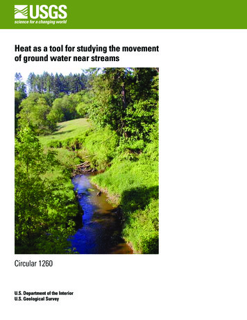
Heat tracing as a hydrological tool near streamscycle (either one day or one year). The penetration of cyclictemperature changes is greater for the case of downward watermovement because the downward-moving water has beenheated and cooled at the land surface. Conversely, the penetration of cyclic temperature changes is less for the case ofupward water movement because the upward-moving groundwater comes from depths that are buffered from temperaturefluctuations at the land surface. This water has a relativelyconstant temperature close to the cyclical average. Maximumand minimum temperatures during a complete cycle (annualor daily) form a ‘temperature envelope’ for a particular site,within which all measured temperature profiles reside. For theannual cycle, January and July profiles typically approximatethe bounds of the envelope. When ground water is flowing intoa gaining stream, the annual envelope collapses toward thestreambed surface. When the stream is losing water to underlying sediments, the envelope expands downward. The samething happens on a smaller scale over the daily cycle, withdawn and afternoon profiles approximating the daily temperature envelope (in which all other, for example hourly, temperature profiles reside).Figure 4 depicts measured temperatures beneath the RioGrande at Albuquerque, New Mexico together with simulatedtemperatures produced by various combinations of hydraulicconductivity and hydraulic gradient [Bartolino and Niswonger,DataOptimal fitKhyd 1 order lowerKhyd 1 order higherReversed gradient3DEPTH, IN METERS5791113158121620TEMPERATURE, IN DEGREES CELESIUS24Figure 4. Measured and modelled temperatures in sedimentsbeneath the Rio Grande. Observed temperature data (dots) arecompared with results of computer simulations (lines) for differenttheoretical values of hydraulic conductivity (Khyd) and hydraulicgradient. These results show the large sensitivity of modeled sediment temperatures to hydraulic parameters.51999]. The figure shows that a hydraulic conductivity of6.7 x 10-6 m/s (0.0000067 meters per second, or about 58centimeters per day) results in simulated temperatures thatclosely match the measured profile. From Darcy’s Law, thetemperature-based estimate of hydraulic conductivity timesthe measured hydraulic gradient provides a robust estimate ofthe water flux. A typical hydraulic gradient is less than 10%(less than a 0.1-m decrease in head per meter of travel). Ratesof ground-water movement are usually a small fraction of thehydraulic conductivity. Changing the hydraulic conductivity(or hydraulic gradient) results in significant changes to thepredicted temperature profile (fig. 4). The large sensitivityof streambed temperatures to hydraulic conditions is readilyapparent, and makes heat a versatile tracer of ground-watermovement. The technical details of applying thermal tracingtechniques are given in the appendices. Appendix A describesthe procurement of data (temperature, heat capacity and thermal conductivity) required to measure and interpret dynamicthermal profiles. Appendix B describes how simulation modelsare constructed and applied to observed measurements, withspecific attention on publicly available computer codes forsimulating the coupled transport of heat and ground water nearstreams.A previewProtecting stream environments and water suppliesrequires an adequate understanding of the interactions betweenstreams and their underlying ground water. The body of thiscircular comprises seven chapters describing the manner inwhich heat has been used to study these interactions in thewestern United States.As described in chapter 2, the Rio Grande is a narrowribbon of water flowing through the parched New Mexicolandscape. The prosperity of the region has depended on theRio Grande since prehistoric times. Current demands on theriver have become so severe that citizens of New Mexico areconsidering their long ignored rights to the Colorado River.The alluvial aquifer beneath the Russian River in northern California is the primary source of water for residents ofSonoma and northern Marin Counties (chapter 3). Three fishspecies are currently listed as endangered, so impacts of waterresources utilization must be carefully monitored (see fig. 5).The Santa Clara River in southern California is the lastnatural stream in Los Angeles County (chapter 4). Maintenance of a healthy river depends intimately on the inter-connectivity of the stream with the adjacent flood plain, whichbroadens westward from the base of the San Gabriel Mountains towards the Pacific Ocean.Tributaries of the Willamette River south of Portland,Oregon, represent spawning habitats for a number of endangered and seagoing fish species. Agriculture in the WillametteValley has shifted from non-irrigated grains to irrigatedorchards, vineyards, and other crops (chapter 5). Changesin stream-water temperature and availability associated with

6Heat as a tool for studying the movement of ground water near streamsFigure 5. Pontoon rafts with fish counting wheels operatingalong the Russian River in coastal northern California. Particular attention to fishery habitat is needed when ground water ispumped near streams.ground-water extraction affect fish populations. Recognitionof these effects has placed new emphasis on quantifying theimpacts of irrigation withdrawals on fish habitats.Trout Creek, California, flows into the southern end ofLake Tahoe, presenting the opportunity to study how streaminteractions with ground water are affected by a lake (chapter6). The exchanges between Trout Creek and shallow groundwater are strongly affected by lake level. Seasonally rising andfalling lake levels create a drastic change in streambed thermalpatterns that, in turn, affect stream ecology.Rillito Creek flows through Tucson, Arizona, providing a main source of recharge to the underlying ground-watersystem. Where and when recharge occurs beneath this rapidlygrowing city is an important uncertainty that affects theregion’s urban planning (chapter 7).Trout Creek in central Nevada is a small stream thatflows down the north side of Battle Mountain (chapter 8). Thestream is typical of thousands of similar streams throughoutthe vast basin and range province. Trout Creek provides anexcellent example for exploring the cumulative importance ofmountain-front streams in providing recharge to regional aquifers. An understanding of mountain-front recharge is essentialfor managing water resources in rugged deserts throughout theworld.As a set, these chapters provide a detailed assessment ofinteractions between surface water and ground water, usingtemperature patterns and their interpretation as a hydrologictool. They also show the manner in which this informationmay be used to better understand and manage biological andwater resources.

Chapter 2The Rio Grande—competing demands for a desert riverJames R. BartolinoIntroductionUTAHCOLORADOThe Middle Rio Grande Basin covers approximatelystudied for a number of years, important gaps remained in the7,900 square kilometers in central New Mexico, encompassunderstanding of the water resources of the basin. In an efforting parts of Santa Fe, Sandoval, Bernalillo, Valencia, Socorro,to fill some of these gaps, the U.S. Geological Survey (USGS)Torrance, and Cibola Counties (“Middle Rio Grande Basin”and other Federal, State, and local agencies conducted anhere refers to the geologic basin defined by the extent ofintensive effort to improve the understanding of the hydrology,deposits of Cenozoic age along the Rio Grande from aboutgeology, and land-surface characteristics of the Middle RioCochiti Dam to about San Acacia). The basin lies in anGrande Basi

channels like these provide information on losses and gains of surface water to and from ground water. Case Creek is one of six study sites in the Willamette Basin where thermal techniques were used to produce estimates of seepage losses to ground water (see Chapter 5).