WIXLIB

XBXrandXAFig. 1.The reachable space is shown as the shaded gray region. Thearrows indicate the possible velocity vectors at each node. Nodes selectedfor extension on the basis of their distance from xrand (xB ) may be difficultto connect from when the system is not small time locally controllable. xAis a better candidate for extension.Algorithm 2 Extend(T )xrand X pdf()xnear arg minxj T ρ(xj , xrand )R δtunew arg minu Ū {ρ(xrand , xnear f (x, u)dt)}Rδtxnew xnear f (x, unew (t))dtT .addVertex(xnew )T .addEdge(unew , xnear xnew )reduction. However, neither approach is able to reduce thedispersion (which must be measured within the reachableset) for uncontrollable systems. Biasing the sampling towardregions close to the goal state has been tried in [14], [15]and [3] with some success. However the sample bias factoris fixed a priori and it can lead to difficulties in non-convexsystems because of the presence of local minima. In [10], ametric accounting for under-actuated dynamics is suggestedbut is specific to the aerial robots example considered there.III. E NHANCEMENTS TO THE RRT A LGORITHMIn this section, we propose three modifications to theoriginal RRT algorithm, all designed to deal with systems thatmay only traverse a small fraction of the entire state space andin which there are no obvious metrics to establish proximityrelationships. Recall that the Voronoi bias coupled with theuse of a uniform distribution decreases the dispersion of thetree nodes in X. However, for uncontrollable systems it maybe impossible to reduce the dispersion of the tree nodes in Xbelow a critical value, which is an unknown constant. Insteadthe goal is to simply find a solution quickly while reducing thedispersion of the tree nodes within the reachable space, R, byusing heuristics to account for the system’s motion constraints.A. Dynamics-based selection of proximal nodeExample 3.1: Consider the trivial exampleẋ1 2,ẋ2 u,(III.1)where u U [1, 2]. The reachable space, which is normallyunknown can easily be computed by hand in this case, andis shown as the shaded region in Fig. 1. A state xrand isgenerated and the planner must select the “closest” tree node,xnear to attempt to connect from. Line 2 of Algorithm 2(traditional RRT) selects xnear xB for extension based onproximity to xrand X, as determined by a distance metricρ that is implicitly assumed to be a Euclidean metric.However, none of the possible velocity vectors at thatstate (indicated as region between the thick arrows) are ableto proceed in the required direction. Despite the fact thatρ(xA , xrand ) ρ(xB , xrand ), xA is actually more suitedto extension because the possible velocity vectors include adirection that moves toward xrand . In addition to testing problems, this situation arises in a variety of robotic applicationswhere the system is nonholonomic (e.g., wheeled carts), andparticularly in systems with constraints on forward velocities(e.g., unmanned aerial vehicles). Ideally both distance andvelocity constraints should be used to estimate a “time toconnection”.To remedy the situation in Fig. 1 we propose replacingρ(xj , xrand ) in Line 2 of Algorithm 2 with a local first orderapproximation of the time-to-go. ρ(xj , xrand )/g if g 0jrand(III.2)t2go (x , x) if g 0where g represents the instantaneous speed with which xrandcan be approached ρ(x, xrand )g max f (x, u) x xj xu ŪIntuitively t2go computes the distance from xj to xrand anddivides by a first order approximation of the speed with whichthe distance can be decreased, giving t2go units of time. Notethat a negative value of g implies that the distance is actuallyincreasing, which can be interpreted as infinite “time-to-go”(to first order). In a given iteration if none of the existingnodes have a finite value for t2go , one can be chosen atrandom or based on some secondary criteria (such as distanceas determined by ρ).From a computational point of view the maximization maybe done by exhaustive search or by exploiting some problemdependent feature. For example if f (x, u) is an affine functionof u and the set U is the Cartesian product of rectangles, themaximization is a linear program in n dimensions which canbe solved efficiently. If no efficient methods exist to computethis quantity, evaluating every node via this method can beintensive. In such a case, t2go can be used as a secondarycriteria to select xnear among the, for example, 10 closestnodes according to the Euclidean metric.We next consider an example that is from the verificationcommunity. Although it is not central to robotics, it hasmany of the properties that are central to multi-agent roboticsystems.Example 3.2: The hybrid automata model of a thermostathas been a popular example in the verification literature [9].Fig. 2 shows the system model. x (x1 , x2 , x3 ) X R3where x1 is the temperature in the room, x2 is the elapsedtime, and x3 is a timer that measures the cumulative amountof time the heater has been on for. The dynamics have twomodes which denote the heater being “on” or “off”. U consistsof uon [2, 4]; and uof f [ 3, 1]. The values uon and

x1 1Metricon: q 1x1 uonx2 1off: q 2x1 uoffuon [2,4]uoff [ 3, 1]x2 1x3 1x3 0T HERMOSTAT E XAMPLE : A COMPARISON OF THE USE OF THE E UCLIDEANMETRIC AND t2go INTRODUCED IN S ECT. III-A, AVERAGED OVER 10x1 3Fig. 2.Euclideant2goNo. ofComputationNodesTime (sec)2284376.41627231TABLE IThe system dynamics of the thermostat.TRIALS ON A1GH Z PC.x13Turn heater offXBlargest VoronoicellXA21Turn heater on1234x2Fig. 3. The solution of the thermostat counter example via the RRT usingthe dynamics-based selection of proximal nodes (Temperature vs. time).uof f represent the possible heating and cooling rates in thetwo modes. The conditions x1 1 and x1 3 enable themode switches of f on and on of f respectively. In [9]a symbolic verification tool is used to answer the question:“After an initialization period of two minutes, is it possiblefor the heater to be on for more than two thirds of the totaltime at any point during the first hour of operation?” Such aquestion may be important from an energy consumption pointof view. Therefore the specification set isS {x X 2/3x2 x3 0 x2 2 0}.The initial conditions were mode “on”, and xo [2 0 0]T .Aside from being a classical verification example, the senariois interesting in its own right. First, the system has quitenontrivial dynamics, since the control inputs do not appearin the right hand side of two of the state equations, or thespecification equations. This, together with the narrow rangeof U , makes the reachable set, R a small subset of X. Theset of possible velocity vectors at every point is very limitedmaking this an ideal example to demonstrate the Dynamicsbased selection of proximal node.First the problem was solved 10 times selecting proximalnodes based on the Euclidean metric ρ; then 10 times withthe Dynamics-based selection function t2go . In all cases, thealgorithm successfully computed a counter example as seenin Fig. 3. Table I shows the computational statistics for twoalgorithms.B. History-based selection of proximal nodeA second situation is shown in Fig. 4 where the traditionalRRT is applied to the system and, after 8 iterations, theresulting tree is shown using dark circles and line segments.Because the reachable set is so small, nodes on the boundarywill tend to have disproportionately large Voronoi regions,such as xA in Fig. 4. When a uniform distribution is used togenerate xrand , most samples will fall outside the reachableset and these boundary nodes will be selected for extensionFig. 4. The reachable space is shown as the shaded gray region, bold circlesand lines are the RRT, and dotted lines are the Voronoi cells. Nodes onthe boundary of the reachable space have disproportionately large Voronoiregions, causing them to repeatedly be selected as xnear .repeatedly. Each time, the same extremal inputs will be used toconnect xA to xrand in vain, instead resulting in xB . Boundarynodes which are repeatedly selected but fail to extend shouldbe penalized to counter balance this Voronoi bias so that theyare less likely to be selected in the future.If a node is selected for extention as xnear in Line 2 ofAlgorithm 2 and the minimization in Line 3 produces an inputunew which has been applied previously, the resulting xnewis already an element of T . When this happens we say thenode has “failed to extend”; and determine the next best unewwhich extends the tree (suggested in [5]).For each xj T we propose storing the number of timesthe node has failed to extend nj . This value can be used tocompute a penalty weight to discourage the repeated selectionof boundary nodes which fail to extend. Let nmin and nmaxbe the least and greatest values of nj in the tree at a giveniteration. The History-based weighting is defined asρ(xj , xrand ) ρminnj nmin ρmax ρminnmax nmin(III.3)where ρmin minxi T ρ(xi , xrand ) and ρmax is defined ina similar manner. These bounds are used to normalize thedistances so that the impact of the second term is not problemdependent. Note that any distance function, including t2go canbe substituted for ρ.Example 3.3: The RRT algorithm is used to find trajectoriesof the linear dynamic system with bounded control inputs inthe form ofẋ Ax Bu b(III.4)H(xj , xrand ; ρ) where x X [ 200 200] [ 200 200] and u U [ 10 10] [ 10 10].Fig. 5 shows trajectories generated by the RRT algorithmusing the Euclidean metric (left) and using the History-basedweighting described above (right). Note that reachable set

1501001000.50.4xB(x; µ, β)1502200x22005050000.30.20.10 60 40 20x0 10 60 40 200No. of cases to fail to extendNo. of cases to fail to extendFig. 5. RRT for a linear system using the Euclidean metric (left) vs. a Historybased selection of proximal node (right). After 5000 nodes the coverage ofthe reachable space is much more dense when using the weighting.302010001000 2000 3000 4000 5000Nodes sorted in descending order 50x510x11302010001000 2000 3000 4000 5000Nodes sorted in descending orderFig. 6. Value of nj for each node (sorted in descending order) using theunweighted Euclidean metric (left) and History-based weighting (right).is small fraction of the environment. The interior of thereachable region with the History-based selection of proximalnode method is much more densely covered than Euclideanmetric. Fig. 6 shows nj for each node in T . Nodes aresorted in descending order to facilitate the visualization. Inthe conventional RRT algorithm, a smaller portion of nodes(on the boundary of the reachable set) have disproportionatelyhigh values of nj .C. Adaptively biased sample generationIntuitively, biasing the sampling distribution for xrand togenerate a disproportionate number of samples inside the set Sis effective when the system is easily steered toward S (i.e. thesystem is output controllable with respect to s(x)). In general,biasing the sample distribution toward the goal can make sensebut it is difficult to decide a priori which problems will benefit.We update the amount of biasing for every Ns iterations ofthe RRT algorithm, where Ns is user defined number. If in agiven iteration ρ(xnear , xrand ) ρ(xnew , xrand ), where ρ isa metric function, we call such an iteration successful becausethe tree has grown toward xrand . We count the number ofsuccessful iterations ns , out of the nβ iterations where randomstates are generated inside the set defined by s(x) 0 andcomputens(III.5)β nβIf xnear is not successful in growing toward xrand inside thespecification set or the best candidate for xnew from xnearis already in a tree in the above test, we eliminate the xnearfrom consideration as xnear for the testing in future iterationsto prevent it from being chosen repeatedly. Values of β closeto unity indicate biasing sample generation inside S has beenbeneficial.Fig. 7.The distribution B(x; µ, β) with µ 0 and various values of β.Our proposed probability density function B(x; µ, β), to beused in Line 1 of Algorithm 2, resembles a Gaussian oversome compact set, a x b N (x; µ, σ(β)) Ct /(b a),a x b(III.6)B(x; µ, β) 0elsewhere N (x; µ, σ(β)) is the Gaussian distribution with meanµ and standard deviation σ(β). The last term, Ct /(b a), isadded to ensure that the area under the curve is equal to one.Ct represents the area of the truncated portions above x band below x aZ aZ Ct N (x; µ, σ)dx N (x; µ, σ)dx. bObviously µ should be selected so that s(µ) 0. Thestandard deviation of N (x; µ, σ(β)) effectively determines thebias and should be computed using β [0, 1]σ(β) (1 β)(σmax σmin ) σmin ,(III.7)where σmax and σmin are user-defined values of the maximumand minimum standard deviations.Fig. 7 illustrates the shape of B(x; µ, β) with different values of β. Distribution (III.6) can be easily implemented usingany random normal generator and rejecting points generatedoutside the compact domain.Example 3.4: We consider a hovercraft in constant altitudeflight with 6 states, x (x1 , x2 , θ, v1 , v2 , ω). The dynamicequations aremv̇1 (f1 f2 ) cos(θ) fx1 air (x, vair (x))mv̇2J ω̇ (f1 f2 ) sin(θ) fx2 air (x, vair (x))(f2 f1 )l τair (x, vair (x))The control inputs are u [f1 f2 ]T (forward actuatingforces) and U [ 10, 10] [ 10, 10]. Forces due to winddisturbances in the x1 , x2 and θ directions are fx1 air , fx2 air ,and τair whose exact expressions are omitted for brevity butare quadratic in the difference between the craft’s velocityand the wind velocity vair and vary with the orientation of thecraft. Note that the state is partitioned into two regions (indoorand outdoor) which define the wind velocity differently:p 22[ αv x2 βv x1 ]T ,p(x1 ) (x2 ) 100 .vair [0 0]T ,(x1 )2 (x2 )2 100

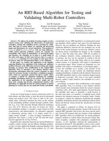
200200150150Algorithm 3 Generate enhanced-RRT: TInitialize RRT: T .addVertex(x0 xinit , n0 0)Global: β 1while (6 x T such that s(x) 0) AND c cmin doenhanced-Extend(T )end whilexx2250225010010050500 500Initial positiongoal regionInitial position50100x11502000 502500goal region50100x1150200250Fig. 8. RRTs of the hovercraft problem with uniform sampling (left) andwith adaptive bias (right).10.8β0.60.40.200Fig. 9.100200300400no. of nodes500600700The evolution of the biasing factor β for the hovercraft problem.We would like to determine if a hovercraft under thesewind conditions can reach some goal zone, S {(x1 , x2 ) [190, 200] [0, 10]}. Note that when outdoors the wind forcesare significantly greater in magnitude than the control inputs,making the system uncontrollable.The initial state is x0 [0 0 0 0 0 0]T . The distribution(III.6) was used to solve the problem 10 times on a 1GHz PC.Fig. 8 shows the solutions of the problem with the uniformsampling distribution and adaptive bias. Fig. 9 shows how βchanges as the algorithm evolves. The adaptive algorithm isable to exploit the situations in which biasing is effective. Asshown in Table II, the adaptive biasing algorithm improvesthe efficiency of RRT method compared to other fixed biasstrategies rather dramatically.Sampling MethodUniformMed. BiasHeavy BiasAdaptive BiasNo. of NodesComputation Time (sec)35561753.51017490.2912408.3678342.5TABLE IIH OVERCRAFT E XAMPLE : A COMPARISON OF THE SAMPLING STRATEGYINTRODUCED HERE (A DAPTIVE B IAS ) TO FIXED - BIAS SAMPLINGSTRATEGIES , AVERAGED OVER10 TRIALS ON A 1GH Z PC.IV. U NIFIED A LGORITHMA. Unified algorithmAlgorithm 3 and 4 present the unification of the enhancements presented in the previous section. Note that, sincemost robotic problems are controllable, the Algorithm 1 canterminate when a solution is found. In our case, it is a distinctpossibility that no solution exists so we impose a secondarytermination criteria. The change in coverage over the trailingN iterations c , measures the growth of the tree. If c dropsbelow some user-defined cmin we terminate the search.Algorithm 4 enhanced-Extend(T )σ (1 β)(σmax σmin ) σminxrand X B(x; µ, β) (see eq.(III.6) )xnear arg minxj T [H(xj , xrand ; t2go )] (seeeq.(III.2),(III.3))R δtunew arg minu Ū [t2go (xrand , xnear f (x, u)dt)]R δtnewnearnewx x f (x, u(t))dtif xnew xj T thennj Ū Ū unewgoto compute unewend ifT .addVertex(xnew , nnew 0)T .addEdge(unew , xnear xnew )reset Ūif Ns iterations thenβ nnβsend ifB. A Multiagent ProblemWe consider a problem where multiple autonomous vehiclesmust guard against an intruder entering a designated area. Thisscenario has applications in games such as “capture the flag”and can be viewed as a variant of the art-gallery problem.It has applications in homeland security where autonomousvehicles (boats, airplanes, ground robots) can be deployed todetect unidentified vehicles entering a cordoned-off area or anexclusion zone.In this example, we examine a circular area, SE guarded by4 robots. Each robot has sensor foot prints which are assumedto be circular with radius Rd for detection and Rc for capture,as shown in Fig. 10. The guarding scheme is shown in Fig. 11.Initially, the guard robots distribute evenly along the perimeterof the exclusion zone. If the intruder enters the detection rangeof a guard robot, the robot pursues the intruder and otherrobots redistribute evenly along the circle CE . If the intruderescapes the detection range of the pursuing robot, the robotreturns to the perimeter and all robots redistribute evenly. Thequestion we wish to answer is as follows. If an intruder or anadversary is allowed to start anywhere in a specified region SI ,and the guard robots are evenly distributed on the circle CE ,can the intruder enter the exclusion zone (SE ) uncaptured? Theanswer to our question can only be found by searching for aninitial condition and a control input function for the intruderwhich drives it into the exclusion zone without crossing any ofthe capture ranges. We assume each of the intruder and guardrobots has 5 states, xi (xi1 , xi2 , θi , v i , ω i ) and 2 control

inputs, ui (ui1 , ui2 ) where x1 and u1 indicate states and inputof the intruder. The dynamics with nonholonomic constraintsare given by:Xi {(xi1 , xi2 , θi , v i , ω i ) R5 (xi1 )2 (xi2 )2 RI2 }B(x (t), Rc ) xi1 )2 (x12 xi2 )2Guard robotdetection range (Rd)CE(IV.1)space X X1 X2 · · · X5 \S5We can i define the free25wherei 2 B(x (t), Rc ) R{(xi1 , xi2 ) (x11IntruderInitial positions for guard robotsInitially, evenly distributedẋi1 v i cos(θi ), ẋi2 v i sin(θi ), θ i ω iv i ui1 , ω̇ i ui2 .iInitial region for intruder (SI) Rc2 }.RIExclusion Zone (SE)capture range (Rc)Fig. 10. Initial conditions for guard robots and intruder. Each robot has adetection range Rd within which the intruder is detected, and capture ragneRc within which the intruder is captured.Then the specification set S is defined byS {x X (x11 )2 (x12 )2 Rs2 }where Rs is the radius of the circle CE .To evenly distribute guard robots along the perimeter, weuse the algorithm proposed in [4]. Each guard robot is subjectto the forceXτ j k ψ 2 (q j ) C q̇ j Fr (q j , q k )(IV.2)k Njwhere q j (xj1 , xj2 ) R2 is the position of robot j, ψ :R2 R is an implicit function description of the perimeterof the exclusion zone that must be guarded and Nj is the setof robots neighboring robot j. Fr is a Coloumb-like repulsiveforce that ensures that the robots do not cluster together, whileC is a constant which provides a viscous damping term. Theforce is applied to a point that is at a finite distance awayfrom a robot to address nonholono

Inspired by the connections between the Testing Problem for complex control systems and the Motion Planning problem, we have recently applied the Rapidly-exploring Random Tree (RRT) algorithm [13] to the testing problem [1], [7] with considerable success. RRT algorithm is an incremental search-ing algorithm which explores state space fast and .