Transcription
Analytic Spherical Harmonic Gradients for Real-Time Rendering withMany Polygonal Area LightsLIFAN WU, University of California, San DiegoGUANGYAN CAI, University of California, San DiegoSHUANG ZHAO, University of California, IrvineRAVI RAMAMOORTHI, University of California, San DiegoFig. 1. We present an analytic formula for spherical harmonic (SH) gradients from uniform polygonal area lights, and show how this new theoretical resultenables scaling Precomputed Radiance Transfer (PRT) to hundreds of area lights. We first compute the lighting SH coefficients and gradients on a sparse 3Dgrid. To evaluate SH coefficients for any intermediate point (vertex), we exploit SH gradients and use accurate Hermite interpolation. Here we render a glossyscene with 713 polygonal (triangular) lights and 1.3M polygons at 36fps. Each light transforms independently (in terms of color, location, orientation etc.),enabling the appearance of textured lights or more complex patterns, and causing significant changes in glossy highlights (compare left and right images).Recent work has developed analytic formulae for spherical harmonic (SH)coefficients from uniform polygonal lights, enabling near-field area lights tobe included in Precomputed Radiance Transfer (PRT) systems, and in offlinerendering. However, the method is inefficient since coefficients need to berecomputed at each vertex or shading point, for each light, even thoughthe SH coefficients vary smoothly in space. The complexity scales linearlywith the number of lights, making many-light rendering difficult. In thispaper, we develop a novel analytic formula for the spatial gradients of thespherical harmonic coefficients for uniform polygonal area lights. The result isa significant generalization, involving the Reynolds transport theorem toreduce the problem to a boundary integral for which we derive a new analyticformula, showing how to reduce a key term to an earlier recurrence for SHcoefficients. The implementation requires only minor additions to existingcode for SH coefficients. The results also hold implications for recent effortson differentiable rendering. We show that SH gradients enable very sparsespatial sampling, followed by accurate Hermite interpolation. This enablesAuthors’ addresses: Lifan Wu, University of California, San Diego, liw086@eng.ucsd.edu; Guangyan Cai, University of California, San Diego, g5cai@ucsd.edu; Shuang Zhao,University of California, Irvine, shz@ics.uci.edu; Ravi Ramamoorthi, University ofCalifornia, San Diego, ravir@cs.ucsd.edu.Permission to make digital or hard copies of all or part of this work for personal orclassroom use is granted without fee provided that copies are not made or distributedfor profit or commercial advantage and that copies bear this notice and the full citationon the first page. Copyrights for components of this work owned by others than theauthor(s) must be honored. Abstracting with credit is permitted. To copy otherwise, orrepublish, to post on servers or to redistribute to lists, requires prior specific permissionand/or a fee. Request permissions from permissions@acm.org. 2020 Copyright held by the owner/author(s). Publication rights licensed to ACM.0730-0301/2020/7-ART1 g PRT to hundreds of area lights with minimal overhead and real-timeframe rates. Moreover, the SH gradient formula is a new mathematical resultthat potentially enables many other graphics applications.CCS Concepts: Computing methodologies Rendering.Additional Key Words and Phrases: analytic gradients, spherical harmonics,area lighting, differentiable renderingACM Reference Format:Lifan Wu, Guangyan Cai, Shuang Zhao, and Ravi Ramamoorthi. 2020. Analytic Spherical Harmonic Gradients for Real-Time Rendering with ManyPolygonal Area Lights. ACM Trans. Graph. 39, 4, Article 1 (July 2020),14 pages. ONIn this paper, we address a fundamental mathematical question,deriving an analytic formula for the spatial gradients of sphericalharmonic (SH) coefficients from a uniform polygonal area light.While both area lights and spherical harmonics are widely used inrendering, to our knowledge, there has been no previous work onfinding analytic SH gradients for them. We believe the result hasimplications for many problems in rendering and beyond.Our immediate practical motivation is for real-time renderingwith precomputed radiance transfer (PRT) [Sloan et al. 2002]. PRTand SH lighting enable dynamic low-frequency environments withrealistic highlights and real-time shading, including soft shadows.Hence, they are widely used in real-time applications like gamesand even in offline rendering [Pantaleoni et al. 2010]. However, theACM Trans. Graph., Vol. 39, No. 4, Article 1. Publication date: July 2020.
1:2 Lifan Wu, Guangyan Cai, Shuang Zhao, and Ravi RamamoorthiPRT method has often been limited to distant environment maps,since area light SH coefficients differ at each vertex on the object.Recent work [Wang and Ramamoorthi 2018] has derived an analytic formula for SH coefficients for a uniform polygonal area light(building on earlier work on irradiance tensors [Arvo 1995; Snyder 1996]), demonstrating area lights in PRT. A similar approachhas also been applied to SH integrals for both offline and real-timerendering [Belcour et al. 2018]. However, those methods requirecomputing the SH coefficients at each integration point (each vertex in PRT), for each light, which precludes easily scaling to largenumbers of lights.An important observation is that the light field from area lights,and hence its SH coefficients, is smooth spatially. This suggests thatthe spatial gradients of SH coefficients are a critical quantity. Althoughgradients and differential methods have recently received significantattention [Li et al. 2018; Zhang et al. 2019], there has so far been littleprevious work in analytically computing SH gradients (as opposed toSH coefficients). One reason may be the challenge of generalizing theSH coefficient derivation, which is already complex, with additionalcomplexity from computing derivatives along each spatial direction.In this paper, we address this long-standing challenge and showhow gradient-based interpolation can enable very sparse spatialsampling, and easy scaling to multiple light sources with minimaloverhead (see Fig. 1). Our specific contributions include:Derivation of Analytic SH Gradient Formula. Our main contribution is the derivation of a novel analytic formula for SH gradients.This is a new result, which is a significant generalization of that forSH coefficients. In particular, we show how to reduce the problemto a boundary integral (§4), where a key term can be reduced to anearlier SH coefficient recurrence (§5). Our practical Algorithm 2 in§6.1 is simple, requiring only a few simple modifications to existingcode for computing analytic SH coefficients.Gradient-Based Interpolation. We demonstrate gradient-based interpolation from a sparse set of samples. An overview of our methodis in Algorithm 1 in §6. We develop a Hermite cubic interpolantthat is consistent with the analytic gradients (§6.2 and Algorithm 4),and more accurate than previous Taylor-series based numericalapproaches [Annen et al. 2004]. Even for rendering with one arealight source, we demonstrate a 2 speedup over explicit analyticcomputation of SH coefficients at each vertex. Our major benefit isfor handling multiple area lights, where we can linearly accumulateSH coefficients and gradients for all lights on a sparse grid withminimal overhead, followed by gradient-based interpolation.Efficient Real-Time Rendering with Multiple Area Lights. We implement our approach within a real-time PRT system. We can handlehundreds of uniform polygonal area lights in real-time, which was notpreviously possible (§7, Figs. 1,10,11). This approach also enableseasily breaking a high-resolution textured light source into uniformpolygonal luminaires, which can be handled with our method.2RELATED WORKPRT and Spherical Harmonics. SH have been widely used in bothreal-time and offline rendering, going back to the work by Cabralet al. [1987]. In particular, they have widely been used in practicefor PRT [Sloan et al. 2002], enabling soft shadows and other lightACM Trans. Graph., Vol. 39, No. 4, Article 1. Publication date: July 2020.transport effects. Approaches based on all-frequency relighting [Nget al. 2003] can be more accurate but have not gained widespreadpractical adoption because of the high precomputation and storage costs. Other analytic methods for area lights, such as the workby Heitz et al. [2016], do not consider shadows. There have beenmany subsequent developments in PRT; we describe only the closest previous work and refer readers to a survey [Lehtinen 2007;Ramamoorthi 2009] for a more thorough introduction.Annen et al. [2004] proposed spherical harmonic gradients formid-range illumination, improving on simply interpolating a smallnumber of locations for incident illumination [Sloan et al. 2002].However, they did not derive an analytic gradient formula, andrequired 2D numerical integration over the area light source, withcomplexity still scaling linearly with the number of lights. In §4and Appendix C, we show that their result is essentially a differentparameterization; our approach enables reduction to a boundaryintegral with an analytic form.Zhou et al. [2005] introduced dynamic scenes and near-field lightsfor all-frequency relighting. Using gradients enables sparser representations, which in turn enable scaling with only a small overheadto hundreds of lights, which was not previously possible. Since ouralgorithm only pertains to the lighting, other benefits such as dynamic scenes, or any other PRT transport algorithm, can easily beincluded. Other all-frequency area light methods include the waveletpropagation approach of [Sun and Ramamoorthi 2009] which alsohandles texture, but the results require approximations and someoperations like out-of-plane light rotation are not permitted. Theirmethod is again limited to a single or small number of lights.Ren et al. [2006] break lights and geometry into spheres and usespherical harmonic exponentiation to enable real-time soft shadowsin more complex dynamic scenes. However, the spherical approximation is not generally suitable for planar area lights (even usingmultiple spheres is a poor approximation of a planar surface fromall directions). Moreover, analytic formulae are provided only forsphere lights. Note that none of the above-mentioned papers compute analytic spherical harmonic gradients, and this computationmay also benefit these approaches in the future.Illumination Gradients. Irradiance and radiance caching [Wardet al. 1988; Křivánek et al. 2005b, 2008] are important techniques forglobal illumination. Greger et al. [1998] introduced the irradiancevolume to precompute and store the irradiance distribution functionin a volumetric grid. Shading at arbitrary points is computed bytrilinearly interpolating from the irradiance volume. In our work, weprecompute and store SH coefficients and gradients in the grid, andperform more accurate Hermite interpolation using the gradients.A series of works [Ward and Heckbert 1992; Křivánek et al. 2005a,2006; Jarosz et al. 2008a,b] exploit irradiance and radiance gradientsto enable sparse sampling of (ir)radiance caching points and accuratevalue interpolation. They use Monte Carlo integration to evaluatethose gradients numerically. In contrast, we derive analytic formulaefor SH gradients. More recently, second-order derivatives (Hessians)have been used for error control of the first-order approximationusing gradients [Jarosz et al. 2012; Schwarzhaupt et al. 2012; Marcoet al. 2018]. It is worth exploring analytic forms of higher orderderivatives in the future.
Analytic Spherical Harmonic Gradients for Real-Time Rendering with Many Polygonal Area LightsHolzschuch and Sillion [1995] developed analytic radiosity gradients with constant and linear emitters. They used Stokes’ theoremto separate the radiosity gradient into two parts: a contour integraland a surface integral. We achieve similar results using the Reynoldstransport theorem [Leal 2007]. Their follow-up work [Holzschuchand Sillion 1998] presented analytic second-order derivatives of theradiosity function, enabling error bounding for hierarchical radiosity algorithms. However, their analysis of the radiosity method onlyhandles diffuse surface patches, while our SH gradients apply toincident lighting and can also be used for glossy surfaces.Differentiable Rendering. Building on early approaches to gradient light transport [Arvo 1994; Ramamoorthi et al. 2007], recentefforts enable differentiating paths including shadows [Li et al. 2018]and radiative transport [Zhang et al. 2019], with different parameterizations [Loubet et al. 2019]. Our method can also be viewedas a differentiable rendering technique, and indeed makes use ofthe Reynolds transport theorem [Leal 2007], also used in the workby Zhang et al. [2019]. However our goals are very different: wecompute SH gradients for PRT, deriving a novel analytic formula. Insights from our paper can be relevant in the future for differentiablerendering and machine learning applications [Liu et al. 2019].Numerical/Automatic Differentiation. For gradient computations,it is possible to use numerical finite differencing. However, thisrequires finding the appropriate step size, and can be noisy andinefficient, as noted in the papers above. It is also possible to useautomatic differentiation (for example, as used in the work by Liet al. [2015]). However, the results are not optimized, and are lessefficient than our analytic gradients. Moreover, we present an explicit analytical derivation, with novel insights, which cannot beachieved with automatic differentiation.3PRELIMINARIESWe first introduce basic background on PRT, spherical harmonics,area lights and differentiating integrals.3.1Reflection Equation and PRTThe simplest version of precomputed radiance transfer (PRT) triesto solve the reflection equation at spatial position x,1 B(x) Li (x, ωi )T (x, ωi ) dωi ,(1)S2where B(x) is the reflected radiance or image intensity, Li (x, ωi ) isthe incoming lighting at x from direction ωi , and we integrate overthe sphere of incoming directions. T (x, ωi ) is the transport functionwhich is precomputed at each vertex in PRT, and encapsulates theBRDF, cosine term and visibility.In this paper, our focus is on lighting, i.e., efficient SH projectionsof Li , rather than the transport T . Any general PRT method can beused to handle the transport function without modifications to therelevant code. In general, Li and T are expanded in (real) sphericalharmonics Ylm (x), which are orthonormal basis functions on the1 For notational simplicity, we assume diffuse reflections and drop dependence ofreflected direction ωo in B and T . In general, we can also handle non-diffuse reflectionsB(x , ωo ) using a glossy PRT extension (see Fig. 1). Since we focus only on lighting L i ,any PRT framework can be supported, including interreflections and dynamic scenes. 1:3unit sphere. Therefore, the integral reduces to a simple summation,ÍÍlB(x) llmaxL (x)Tlm (x),(2) 0 m l lmwhere Llm and Tlm are spherical harmonic coefficients for theÍlighting and transport respectively (with L l ,m Llm Ylm andÍT l ,m Tlm Ylm ). We typically consider l max 8 in this paper,involving 81 SH terms; the summation can be computed at each vertex x as a dot-product of lighting and transport coefficient vectorsin graphics hardware for each color channel.In the original PRT formulation for distant environment maps,lighting is independent of spatial position x and the lighting coefficients Llm can be computed once for each frame, while transportcoefficients Tlm (x) are precomputed and stored. In our case, fornear-field area lighting, Llm (x) changes at each spatial location.3.2Spherical HarmonicsSpherical harmonics (SH) are a set of orthogonal functions Ylmdefined on the unit sphere S2 . Let ω (θ, ϕ) (x, y, z) be aunit direction on S2 . The forms of the real SH basic functions aresummarized in Appendix A. In particular, zonal harmonics (ZH)Yl 0 (ω) Kl Pl (cos θ ) are a subsetq of SH basis functions for m 0,where the normalization Kl 2l4π 1 and Pl is the Legendre polynomial of degree l. Zonal harmonics are radially symmetric aroundthe z-axis. To represent a ZH basis function that is centered aroundan arbitrary axis ωc , we write the rotated ZH using dot products:Yl 0 (ω · ωc ) Kl Pl (ω · ωc ).As pointed out by Nowrouzezahrai et al. [2012], any SH basisfunction Ylm can be sparsely factorized into a sum of rotated ZHbasis functions,Í(3)Ylm (ω) j αlm,j Yl 0 (ω · ωl ,j ),where ωl ,j represents the central direction of each rotated ZH lobeand αlm,j is its corresponding weight. Theoretically, to representeach band-l SH basis function, 2l 1 rotated ZH lobes are required.However in practice, the ZH lobes can be shared across all bands(Appendix B), resulting in a sparse weight matrix αlm,j and faster SHrotation.3.3Analytic Spherical Harmonic CoefficientsGiven a polygonal light source A with unit intensity, we denote itsprojection onto a unit sphere centered at the shading point x asQ(x). The SH coefficients of this area light source with respect to xare given by integrating the SH basis functions over Q, Llm (x) Ylm (ω) dω.(4)Q (x )By applying the zonal harmonic factorization (Eq. (3)) to Ylm , theSH coefficients can be rewritten as Õ mªLlm (x) αl ,j Yl 0 (ω · ωl ,j ) dωQ (x ) j« Õm αl ,jYl 0 (ω · ωl ,j ) dω .(5)jQ (x ) {z : Ll ,j (x )}ACM Trans. Graph., Vol. 39, No. 4, Article 1. Publication date: July 2020.
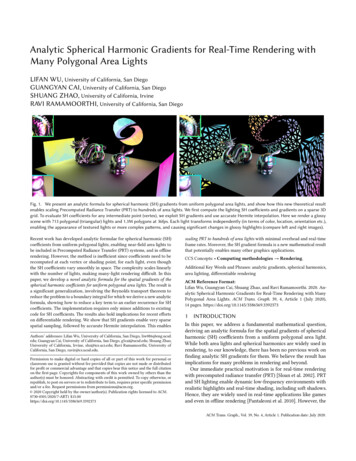
1:4 Lifan Wu, Guangyan Cai, Shuang Zhao, and Ravi RamamoorthiTherefore, computing Llm (x) boils down to computing the ZH coefficients Ll ,j (x). Belcour et al. [2018] further represented the ZHcoefficient as the sum of cosine-power integrals and found analytic solutions for these integrals over spherical polygons. Wangand Ramamoorthi [2018] derived analytic ZH coefficients by applying Stokes’ Theorem to convert surface integrals to boundaryintegrals. The boundary integrals are further solved using the recurrence relations of Legendre polynomials, which are also usedin our derivation. However, our approach is different, in terms offinding the SH gradients, which we reduce to a novel boundaryintegral by differentiating the surface integral for ZH coefficients. Acrucial insight helping us to find the analytic formula is in reducinga key term to the earlier ZH coefficient recurrence, which involvesminimal overhead to evaluate coefficients and gradients jointly.3.4Differentiating IntegralsIn this paper, our goal is to find the SH spatial gradients x Llm (x),which we will often denote simply as Llm (x). This reduces todifferentiating the integral on the right-hand side (RHS) of Eq. (4).To this end, we leverage the Reynolds transport theorem whichoriginates in fluid mechanics [Leal 2007] and generalizes the Leibnizintegral rule for differentiation under the integral operator.Let Ω(π ) be an n-dimensional manifold parameterized by π . Weare interested in differentiating the integration of a function f overthe region Ω(π ). The partial derivative with respect to π can beexpressed as Û f d Ω(π ), πf dΩ(π ) fÛ dΩ(π ) ⟨n, x⟩Ω(π )Ω(π ) Ω(π )(6)where π : and fÛ : π f . The differentiation result has twoπparts. The first one is an integral on the original domain Ω(π ). Theother one is a boundary integral on the (n 1)-dimensional region Ω(π ). For its integrand, we define xÛ : π x, n is the normaldirection at each x Ω(π ) and points towards the exterior byconvention, and ⟨·, ·⟩ is the dot product of two vectors.Recent work in differentiable rendering [Li et al. 2018; Zhanget al. 2019] have already shown the significance of the boundaryintegral for correctly evaluating geometric derivatives. Later in §4and §5, we will see the boundary integral also leads to significantformula simplification and enables the analytic derivation.4DIFFERENTIATING SPHERICAL HARMONICCOEFFICIENTSIn this section, we will use the Reynolds transport theorem to differentiate the SH coefficients for area lights, showing that SH gradientscan be computed from boundary integrals. In §5 we will furtherderive our key result, an analytic formula. In §6 we develop our SHgradient (jointly with SH coefficients) evaluation algorithm and thegradient-based interpolation method, showing how to handle multiple area light sources. While the derivation is somewhat involved,the actual algorithm involves only a few simple modifications toprevious code for SH coefficients. Readers interested primarily inimplementation may wish to first browse §6 and Algorithms 1 and 2.Let A (p 1, p 2, . . . , p N ) be a uniform polygonal light sourcewith N points in R3 and x be the shading point where we wantACM Trans. Graph., Vol. 39, No. 4, Article 1. Publication date: July 2020.(a)(b)Fig. 2. (a) Illustration of the spherical projection for a triangle light. (b)When the shading point x moves by xÛ (equivalent to the area light movesby xÛ ), the projected spherical polygon also changes accordingly.to evaluate the incident radiance (see Fig. 2-a). Note that Q(x) (ω1, ω2, . . . , ω N ) is a spherical polygon obtained by projecting Aonto the unit sphere S2 centered at x (see Fig. 2-a), where ωi p i x2 p i x . Both Q(x) and its boundary (which consists of arcs on S ) Q(x) {ωi ωi 1 i 1, . . . , N } may vary with x.4.1Spherical Harmonic GradientGiven a shading point x (x, y, z), we define the SH gradient asthe spatial gradients with respect to x, Llm (x) ( x Llm (x), y Llm (x), z Llm (x)).(7)Without loss of generality, we will focus on one of the spatial partial derivatives z Llm (x) in the following derivations. The othergradient components can be evaluated in the same way.To evaluate the SH coefficient in Eq. (4), the SH basis functionis integrated over a varying domain Q(x) as the shading point xchanges. By applying the Reynolds transport theorem to the righthand side (RHS) of Eq. (4), we can write the partial derivative as zYlm (ω) dω z [Ylm (ω)] dω Q (x )Q (x ) Û lm (ω) dℓ(ω).⟨n , ω⟩Y(8) Q (x )The first integral on the RHS vanishes, because the SH basis function is independent of the shading point position so z [Ylm (ω)] 0.The second integral is due to the moving boundary Q(x) as xvaries (see Fig. 2-b). For every ω Q(x), dℓ(ω) represents the arclength measure. The normal vector n is in the tangent space ofω S2 and perpendicular to the boundary curve. We denote ωÛ asthe change rate of the boundary location ω with respect to z, i.e.ωÛ z ω. Let y A be a point on the polygonal light boundary.Further, the shading point x has a change rate xÛ (0, 0, 1). Wecan establish the following relation between the change rates (seeFig. 3),ωÛ z4.2 y x xÛ xÛ ω ω,. y x y x y x (9)Reduction to Edge/Arc IntegralsThe previous subsection shows that the spatial partial derivativecan be simplified as Û lm (ω) dℓ(ω), z Llm (x) ⟨n , ω⟩Y(10) Q (x )
Analytic Spherical Harmonic Gradients for Real-Time Rendering with Many Polygonal Area LightsFig. 3. Evaluating the change rate of ω. We first project xÛ to the unit xÛsphere, then obtain ωÛ by extracting the component of y x that is perpendicular to ω.which is a 1D integral on the spherical polygon edges.We now decompose the boundary integral into a sum of arc integrals for each arc ωi ωi 1 Q(x),N ÕÛ lm (ω) dℓ(ω) . z Llm (x) ⟨ni , ω⟩Y(11) 1:5while the integrand is independent. Therefore, the integral of thedifferentiated quantity (first integral on the RHS of Eq. (8)) is zero.Although both methods result in equivalent solutions, they havedifferent algorithmic implications. In the work by Annen et al. [2004],they need to numerically integrate functions in 2D, even though theintegrand can be evaluated analytically or by automatic differentiation. On the other hand, our parameterization results in dimensionreduction. The 1D integrals can not only be evaluated numericallyin a more efficient way, but also lead to analytic solutions. Differentapplications may prefer specific parameterizations. For example, indifferentiable rendering [Li et al. 2018; Zhang et al. 2019; Loubetet al. 2019], one wants to avoid the boundary integration as much aspossible, because the gradient estimation requires additional effortfor edge sampling. Further, the edge integrals they evaluated aretoo complex to have analytic solutions. In contrast, we prefer toreduce SH gradients to edge integrals. The dimension reduction onthe integral domain makes the analytic derivation much easier. i ω i 1i 1 ω {z}5(i ) : G lm For every ω ωi ωi 1 , it has the same normal directionωi ωi 1.(12)ni ωi ωi 1 Further, the edge integral can be parameterized with the radianangle t [0,Ti ], Ti arccos (ωi · ωi 1 ) asω(t) ωi cos t λ sin t,In this section, we will show how to solve SH gradients analytically.First, we use ZH factorization [Nowrouzezahrai et al. 2012], seeEqs. (3, 5), to rewrite Eq. (14) in terms of ZH integrals (we focus onone edge in the following derivations),(i)Glm (13)Û can be evaluatedwhere λ ni ωi . The direction change rate ω(t)using Eq. (9). The arc length measure dℓ(ω) is equal to dt since thesphere radius is one. In summary, we can rewrite the arc integralsin Eq. (11) as simple 1D integrals, Ti(i)ÛGlm ⟨ni , ω(t)⟩Y(14)lm (ω(t)) dt .0(i)At this point, it would be possibly to simply evaluate Glm efficiently using 1D numerical quadrature rules.2 However, we will goeven further, deriving a fully analytic recurrence formula in §5.Discussion. The reduction of area light computations to edgeintegrals over the bounding arcs is common, but previous workhas used Stokes’ theorem for polynomial or spherical harmoniccoefficients [Snyder 1996; Wang and Ramamoorthi 2018]. Our use ofthe Reynolds transport theorem to reduce the gradients to boundaryintegrals is a novel approach, to the best of our knowledge.Annen et al. [2004] developed a semi-analytic solution to SHgradients. We show in Appendix C that their results can also bederived from the Reynolds transport theorem, but using a differentparameterization. In their case, the integration domain is independent of the varying parameters. As a result, the boundary integral(second integral on the RHS of Eq. (8)) becomes zero after differentiating with the Reynolds transport theorem. On the other hand,we use a parameterization such that the integration domain varies2 Note that the integrand is smooth and low-dimensional (1D), so Monte Carlosampling is not required; a standard integration rule like Simpson’s or a higher-orderquadrature scheme could be employed. This may be desirable in some applications.ANALYTIC FORMULAÕjαlm,j TiÛ⟨ni , ω(t)⟩Yl 0 (ω(t) · ωl ,j ) dt .(15)0 {z}(i ) : G l ,jThe weights αlm,j and central directions ωl ,j of the ZH lobes canbe precomputed. Now, the problem reduces to how to evaluate the(i)integral Gl ,j analytically.The input of our method includes the edge endpoints pi and pi 1 ,the shading point x, its change rate xÛ that equals (0, 0, 1) whendifferentiating with respect to z, and the central direction ωl ,j ofthe j-th ZH lobe. Briefly, the derivation involves simplifying theintegrand, rearranging terms and reducing to the known recurrencerelations of Legendre polynomials.5.1Solving for Gl(i),jTransforming to Local Frame. We seek to represent the integrand(i)Ûof Gl ,j by a function of t, i.e., д(t) ⟨ni , ω(t)⟩Yl 0 (ω(t) · ωl ,j ), andsimplify it as much as possible. First, we translate the edge pi pi 1 by x so that the shading point is at the origin. We denote the distancesfrom the shading point to the edge endpoints as ℓi pi x and ℓi 1 pi 1 x . The arc ωi ωi 1 is represented by twounit vectors ωi and ωi 1 . Then, we build a local frame (ωi , λi , ni ),where ni and λi are defined in Eqs. (12, 13). We transform all therelated vectors ωi , ωi 1, and ωl ,j into this local frame by a rotationoperator R(u) (u ·ωi , u · λi , u ·ni ). One benefit is that expressionsof ω(t) are simpler after rotation: R(ω(t)) (cos t, sin t, 0), becausethe edge is completely in the xy-plane and ωi aligns with the x-axis.Moreover, the function value д(t) is unchanged since the dot productis invariant under rotation.ACM Trans. Graph., Vol. 39, No. 4, Article 1. Publication date: July 2020.
1:6 Lifan Wu, Guangyan Cai, Shuang Zhao, and Ravi RamamoorthiÛSimplifying ⟨ni , ω(t)⟩.To evaluate this term, we can expand andsimplify it using Eq. (9): xÛ xÛÛ⟨ni , ω(t)⟩ ni , ⟨ni , ω(t)⟩ ω(t), y(t) x y(t) x 1Û ⟨ni , x⟩,(16) y(t) x because ni is perpendicular to ω(t). Assuming ni (n x , ny , nz ), weÛ nz . Then, it remains to find ℓ(t) y(t) x .know that ⟨ni , x⟩We denote y(t) x ℓ(t)ω(t) as the intersection point of pi pi 1and the ray with direction ω(t) starting at x. The solution can befound by solving a linear system, sin t sin (t Ti ) 1ℓ(t) sinTi .(17)ℓi 1ℓiRecall that ℓi and ℓi 1 are the distances to area light vertices pi andpi 1 respectively, from the shading point x (corresponding to ℓ(0)and ℓ(Ti )). We provide the detailed derivation in Appendix D.1.To sum up, Eq. (16) can be written as nzsin t sin (t Ti )Û⟨ni , ω(t)⟩ .(18)sinTi ℓi 1ℓiSimplifying Yl 0 (ω(t) · ωl ,j ). Given a precomputed central direction ωl ,j , we denote the vector after rotation as R(ωl ,j ) (c x , cy , c z ). The ZH basis function can be written asYl 0 (R(ω(t)) · R(ωl ,j )) Kl Pl (c x cos t cy sin t).Rearranging Terms. Despite our simplifications to the integrand,it remains nontrivial to evaluate the integrals in Eq. (20) analytically.Fortunately, for h(t) c x cos t cy sin t, the integral hPl (h) dt doeshave a closed-form solution, which can be deri
implications for many problems in rendering and beyond. Our immediate practical motivation is for real-time rendering with precomputed radiance transfer (PRT) [Sloan et al. 2002]. PRT and SH lighting enable dynamic low-frequency environments with realistic highlights and real-time shading, including soft shadows.