![Advanced Analytics In Business [D0S07a] Big Data Platforms .](/img/28/3-20-20supervised-20learning.jpg)
Transcription
Advanced Analytics in Business [D0S07a]Big Data Platforms & Technologies [D0S06a]Supervised Learning
OverviewRegressionLogistic regressionK-NNDecision and regression trees2
The analytics process3
RecallPredictive analytics (supervised learning)Predict the future based on patterns learnt from past dataClassification (categorical) versus regression (continuous)You have a labelled data set at your disposalDescriptive analytics (unsupervised learning)Describe patterns in dataClustering, association rules, sequence rulesNo labelling requiredFor supervised learning, our data set will contain a label4
Classification (categorical target)Churn prediction: churn yes/noCredit scoring: default yes/noFraud detection: suspicous yes/noResponse modeling: customer buys yes/noPredictive maintenance: needs check yes/noMost classification use cases use a binary categorical variableWhat if there are more than two outcomes "multiclass" classificationNot all techniques can handle thisBut "tricks" exist to set up multiclass problems using binary classification techniquesWhat if the outcomes are ordered "ordinal" classification"Tricks" exist to set up ordinal problems using binary classification techniquesWhat if more than two outcomes are possible at the same time "multi-label" classificationHere too, simple transformative approaches existWe'll visit these later on5
Regression (continuous target)Customer lifetime value (CLV) modelingLoss forecasting (LGD)Price forecasting6
Defining your targetRecommender system: a form of multi-class? Multi-label?Survival analysis: instead of yes/no predict the "time until yes occurs"Oftentimes, different approaches are possibleRegression, quantile regression, mean residuals regression?Or: predicting the absolute value or the change?Or: convert manually to a number of bins and perform classification?Or: reduce the groups to two outcomes?Or: sequential binary classification ("classifier chaining")?Or: perform segmentation first and build a model per segment?7
Regression8
Regressionhttps://xkcd.com/605/9
Linear regressionNot much new here.y β0 β1 x1 β2 x2 . ϵ with ϵ N (0, σ)Price 100000 100000 * number of bedroomsβ0 : mean response when x⃗ 0 (y-intercept)β1 : change in mean response when x1 increased by one unitHow to determine the parameters?argminβ ⃗ ni 1 (yi y i )2 : minimize sum of squared errors (SSE)With standard error σ SSE/nOLS: "Ordinary Least Squares". Why SSE though?10
Logistic regression11
Logistic regressionClassification is solved as well?Customer Age Income Gender . ResponseJohn301200MNo 0Sophie242200FNo 0Sarah531400FYes 1David481900MNo 0Seppe35800MYes 1y β0 β1 age β2 income β3 genderBut no guarantee that output is 0 or 1Okay fine, a probability then, but no guarantee that outcome is between 0 and 1 eitherTarget and errors also not normally distributed (assumption of OLS violated)12
Logistic regressionWe use a bounding function to limit theoutcome between 0 and 1:f (z) 11 e z (logistic, sigmoid)Same basic formula, but now with the goal ofbinary classificationTwo possible outcomes: either 0 or 1, no or yes – a categorical, binary label, not continuousLogistic regression is thus a technique for classification rather than regressionThough the predictions are still continuous: between [0,1]13
Logistic regressionLinear regression with a transformation such that the output is always between 0and 1, and can thus be interpreted as a probability (e.g. response or churnprobability)P (response yes age, income, gender) 1 P (response no age, income, gender) 11 e (β0 β1 age β2 income β3 gender)Or:ln(P (response yes age, income, gender)) β0 β1 age β2 income β3 genderP (response no age, income, gender)14
Logistic regressionCustomer Age Income Gender . ResponseJohn301200MNo 0Sophie242200FNo 0Sarah531400FYes 1David481900MNo 0Seppe35800MYes 1 Our first predictive model: aformulaNot very spectacular, but note:Easy to understandEasy to constructEasy to implement11 e (0.10 0.22age 0.05income 0.80gender) Customer Age Income Gender .ResponseScoreWill441500M0.76Emma281000F0.44In some fields/settings, the endresult will be a logistic model"extracted" from more complexapproaches15
Logistic regressionIterative approach, but very fastEasy to interpret and understandStatistical rigor, a "well-calibrated" classifierStill a good rule of thumb is to start with logistic regressionLinear decision boundary, though interaction effects can be taken into the model (andexplicitely; allows for investigation)Relatively robust to noise, though sensitive to outliersCategorical variables need to be converted (e.g. using dummy encoding as the most commonapproach, though recall ways to reduce large amount of dummies)Somewhat sensitive to the curse of dimensionality.16
Regularization17
Stepwise approachesStatisticians love parsimonious modelsIf a "smaller" model works just as well as a "larger" one, prefer the smaller oneAlso: "curse of dimensionality"Most statistical techniques don't like dumping in your whole feature set all atonceSelection based approaches (build up final model step-by-step):Forward selectionBackward selectionHybrid (stepwise) selectionSee MASS::stepAIC , leaps::regsubsets , caret , or simply step in RNot implemented by default in Python (neither scikit-learn or statsmodels )What's going on?18
Stepwise approachesTrying to get the best, smallest model given some information about a largenumber of variables is reasonableMany sources cover stepwise selection methodsHowever, this is not really a legitimate situationFrank Harrell (1996):It yields R-squared values that are badly biased to be high, the F and chi-squared tests quotednext to each variable on the printout do not have the claimed distribution. The method yieldsconfidence intervals for effects and predicted values that are falsely narrow (Altman andAndersen, 1989). It yields p-values that do not have the proper meaning, and the propercorrection for them is a difficult problem. It gives biased regression coefficients that needshrinkage (the coefficients for remaining variables are too large (Tibshirani, 1996). It hassevere problems in the presence of collinearity. It is based on methods (e.g., F tests for nestedmodels) that were intended to be used to test prespecified hypotheses. Increasing the samplesize does not help very much (Derksen and Keselman, 1992). It uses a lot of cs/stepwise-regression-problems/)““19
Stepwise approachesSome of these issues have / can be fixed (e.g. using proper tests), but.Developing and confirming a model based on the same dataset is called data dredging.Although there is some underlying relationship amongst the variables, and strongerrelationships are expected to yield stronger scores, these are random variables and therealized values contain error. Thus, when you select variables based on having better realizedvalues, they may be such because of their underlying true value, error, or both. True, usingthe AIC is better than using p-values, because it penalizes the model for complexity, but theAIC is itself a random variable (if you run a study several times and fit the same model, theAIC will bounce around just like everything else).““This actually already reveals something we'll visit again when talking aboutevaluation!Take-away: use a proper train-test setup!20
RegularizationSSEM odel1 (1 1)2 (2 2)2 (3 3)2 (8 4)2 16SSEM odel2 (1 1)2 (2 2)2 (3 5)2 (8 8)2 821
RegularizationKey insight: let us introduce a penalty on the size of the weightsConstrained, instead of less parameters!Makes the model less sensitive to outliers, improves generalizationLasso and ridge regression:Standard: y β0 β1 x1 . βp xp ϵ with argminβ ⃗ ni 1 (yi y i )2Lasso regression (L1 regularization): argminβ ⃗ ni 1 (yi y i )2 λ pj 1 βj Ridge regression (L2 regularization): argminβ ⃗ ni 1 (yi y i )2 λ j 1 βj2pNo penalization on the intercept!22
Lasso and ridge /stat508/lesson/5/5.123
Lasso and ridge regressionLasso will force coefficients to become (close to) zero, ridge only to keep them within boundsVariable selection for free with lassoWhy ridge, then? Easier to implement (slightly) and faster to compute (slightly), or when youhave a limited number of variables to begin withIn practice, however, lasso is preferred, tends to work well even with small sample sizesDrawback: if group of correlated variables is present, lasso selects one at randomHow to pick a good value for lambda: cross-validation! (See later)Works both for linear and logistic regression, concept of L1 and L2 regularization also pops upwith other model types (e.g. SVM’s, Neural Networks) and fields:Tikhonov regularization (Andrey Tikhonov), ridge regression (statistics), weight decay (machine learning), theTikhonov–Miller method, the Phillips–Twomey method, the constrained linear inversion method, and the methodof linear regularizationNeed to normalize variables befhorehand to ensure that the regularisation term λregularises/affects the variable involved in a similar manner!MATLAB always uses the centred and scaled variables for the computations within ridge. Itjust back-transforms them before returning them.““24
Elastic netEvery time you have two similar approaches, there's an easy paper opportunityby proposing to combine them (and giving it a new name)nppi 1j 1j 1argminβ ⃗ (yi y i )2 λ1 βj λ2 βj2Combine L1 and L2 penaltiesRetains benefit of introducing sparsityGood at getting grouping effectsImplemented in R and Python (check the documentation: everybody disagrees on how to callλ1 and λ2 )Grid search on two parameters necessaryLasso parameter will be the most pronounced in most practical settings25
Some other forms of regression26
Non-parametric regression"Non-parametric" being a fancy name for "nounderlying distribution assumed, purely datadriven"“Smoothers” such as LOESS (locally weightedscatterplot smoothing)Does not require specification of a function to fit a model, onlya “smoothing” parameterVery flexible, but requires large data samples (because LOESSrelies on local data structure to provide local fitting), does notproduce a regression functionTake care when using this as a “model”, more an exploratorymeans!27
Generalized additive models(GAMs), similar concept as normal regression, but uses splines and other given smoothingfunction in a linear combinationBenefit: capture non-linearities by smooth functionsFunctions can be parametric, non-parametric, polynomial, local weighted mean, .Very flexible, best of both worlds approachDanger of overfitting: stringent validation requiredy β0 f1 (x1 ) . fp xp ϵTheoretical relation to boosting (which we'll discuss later)Very nice technique but not that well knownaerosolve - Machine learning for humansA machine learning library designed from the ground up to be human friendly.A general additive linear piecewise spline model. The training is done at a higher resolutionspecified by num buckets between the min and max of a feature's range. At the end of eachiteration we attempt to project the linear piecewise spline into a lower dimensional function suchas a polynomial spline with Dirac delta endpoints.““28
Generalized additive modelsHenckaerts, Antonio, et al., 2017:log(E(nclaims)) log(exp) β0 β1 coverageP O β2 coverageF O β3 f ueldiesel f1 (ageph) f2 (power) f3 (bm) f4 (ageph, power) f5 (long, lat)29
Decision trees30
Decision treesBoth for classification and regressionWe'll discuss classification firstBased on recursively partioning thedataSplitting decision: How to split a node?Age 30, income 1000, status married?Stopping decision: When to stop splitting?When to stop growing the tree?Assignment decision: How to assign a label outcome in the leaf nodes?Which class to assign to the leave node?31
Terminology32
ID3ID3 (Iterative Dichotomiser 3)Most basic decision tree algorithm, by Ross Quinlan (1986)Begin with the original set S as the root nodeOn each iteration of the algorithm, iterate through every unused attribute of the set S andcalculate a measure for that attribute, e.g. Entropy H(S) and Information Gain IG(A,S)Select the best attributeSplit S on the selected attribute to produce subsetContinue to recurse on each subset, considering only attributes not selected before (for thisparticular branch of the tree)Recursion stops when every element in a subset belongs to the same class label, or there are nomore attributes to be selected, or there are no instances left in the subset33
ID334
ID335
ID336
Impurity measuresWhich measure?Based on impurity Minimal impurity Also minimal impurity Maximal impurity37
Impurity measuresIntuitively, it's easy to see that: Is better than: But what about: We need a measure38
EntropyEntropy is a measure of the amount of uncertainty in a data set (informationtheory)H(S) x X p(x)log2 (p(x)) with S the data (sub)set, X the classes(e,g, {yes, no}), p(x) the proportion of elements with class x over S When H(S) 0, the set is completely pure (alle elements belong to the same class)39
EntropyFor the original data set, we get:#yes #no x yes x no Entropy95-0.41-0.530.9440
Information gain We can calculate the entropy of the original set and all the subsets, but how tomeasure the improvement?Information gain: measure of the difference in impurity before and after the splitHow much uncertainty was reduced by a particular split?IG(A, S) H(S) t T p(t)H(t) with T the set of subsets obtainedby splitting the original set S on attribute A and p(t) t / S 41
Information gainOriginal set S:#yes #no x yes x no Entropy95-0.41-0.530.94Calculate the entropy for all subsets created by all candidate splitting bset #yes #no x yes x no -0.40.59Strong33-0.50-0.501Weak62-0.31-0.50.81042
Information gainIG(A, S) H(S) t T p(t)H(t)545IG(outlook, S) 0.94 - ( 140.97 140.00 140.97) 0.94 - 0.69 0.25 highest IGIG(temperature, S) 0.03IG(humidity, S) 0.15IG(wind, S) 0.05#yes #no x yes x no HumidityWindSubset #yes #no x yes x no -0.40.59Strong33-0.50-0.501Weak62-0.31-0.50.81043
ID3: after one split44
ID3: continueRecursion stops when every element in a subset belongs to the same class label,or there are no more attributes to be selected, or there are no instances left in thesubset45
ID3: final treeAssign labels to the leaf nodes: easy -- just pick the most common class46
Impurity measuresEntropy (Shannon index) is not the only measure ofimpurity that can be usedEntropy: H(S) x X p(x)log2 (p(x))Gini diversity index: Gini(S) 1 x X p(x)2Gini gain similar as information gain with Entropy (use Gini(S) instead ofH(S))Not very different: Gini works a bit better for continuous variables (see after) and is a little fasterMost implementations default to this approachClassification error: ClassErr(S) 1 maxx X p(x)Something to think about: why not use accuracy directly? Or another metric ofinterest such as AUC or precision, F1, .?47
Summary so farUsing the tree to predict new labels is just as easy as using a regression formula: just follow thequestions in the tree and look at the outcomeEasy to understand, easy (for a computer) to constructCan be easily expressed as simple IF.THEN rules as well, can hence be easily implemented inexisting programs (even as a SQL procedure)Fun as background research: algorithms exist which directly try to introduce prediction modelsin the form of a rule base, with RIPPER (Repeated Incremental Pruning to Produce ErrorReduction) being the most well known. It's just as old and leads to very similar models, but hassome interesting differences and is (nowadays) not widely implemented or known anymore48
/rules.html49
Problems still to solveID3 is greedy: it never backtracks (i.e.retraces on previous steps) during theconstruction of the tree, it only movesforwardThis means that global optimality of the tree is notguaranteedAlgorithms exist which overcome this (see e.g.evtree package for R), though they're often slowand do not give much better results (greedy is goodenough)A bigger problem however is the fact that wedo not have a way to tackle continuousvariables, such as temperature 21, 24, 26,27, 30, .Another big problem is that the "grow for aslong as you can" strategy leads to trees whichwill be horribly overfitting!50
Spotting overfittingNote that this is a good motivating case to illustrate the difference between"supervised methods for predictive analytics" or "for descriptive analytics"51
C4.5Also by Ross QuinlanExtension of ID3Main contribution: dealing with continuous variablesCan also deal with missing variables. The original paper describes that you just ignore themwhen calculating the impurity measure and information gain, though most implementations donot implement this!Also allows to set importance weights on attributes (biasing the information gain, basically)Describes methods to prune trees52
C4.5: continuous variablesSay we want to split on temperature 21, 24, 26, 27, 30, .Obviously, using the values as-is would not be a good ideaWould lead to a lot of subsets, many of which potentially having only a few instancesWhen applying the tree on new data: the chance of encountering a value which was unseenduring training is much higher than for categoricals, e.g. what if temperature is 22?Instead, enforce binary splits by:Splitting on temperature 21 -- two subsets (yes, no) -- and calculate the information gainSplitting on temperature 24 -- two subsets (yes, no) -- and calculate the information gainSplitting on temperature 26 -- two subsets (yes, no) -- and calculate the information gainSplitting on temperature 27 -- two subsets (yes, no) -- and calculate the information gainAnd so on.Important: only the distinct set of values seen in the training set are considered, though somepapers propose changes to make this a little more stable53
C4.5: preventing overfittingEarly stopping: stop based on a stop criterionE.g. when number of instances in subset goes below a thresholdOr when depth gets too highOr: set aside a validation set during training and stop when performance on this set starts todecrease (if you have enough training data to begin with)54
C4.5: preventing overfittingPruning: grow the full tree, but then reduce itMerge back leaf nodes if they add little power to the classification accuracy"Inside every big tree is a small, perfect tree waiting to come out." --Dan SteinbergMany forms exist: weakest-link pruning, cost-complexity pruning (common), etc Oftentimes governed by a "complexity" parameter in most implementations55
C5 (See5)Also by Ross QuinlanCommercial offeringFaster, memory efficient, smaller trees, weighting of cases and supplying misclassification costsNot widely adopted only recently made open source, better open source implementationsavailableSupport for boosting (see next course)56
A few final insightsBinary splitsRemember the continuous splits: binary split (x split yes / no)Couldn't we do the same for categorical values?E.g. humity high yes/no?We can, and most (good) implementations indeed do so (Weka is a weird exception). This infact also prevents a bias issue in the information gain measure: by default, it is biased to prefersplits leading to more subsetsThis can make the tree deeper, but this is not a big issueNote that we can now encounter the same attribute multiple times in the "path" through a treetowards a leaf nodeConditional inference trees provide another method to avoid this bias by using a significancetest procedure in order to select variables instead of selecting the variable that maximizes aninformation measureSome implementations have proposed three-way splits (yes / no / NA) but not manyThis means that you will have to treat missing valuesHowever, trees are surprisingly robust to other issues, such as outliers57
A few final insightsRemember to prevent overfitting treesBut a deep tree does not necessarily mean that you have a problemAnd a short tree does not necessarily mean that it's not overfittingHowever, note that it is now very likely that your leaf nodes will not becompletely pure (i.e. not containing 100% yes cases or no cases)How to assign an outcome?Easy, take the majority classWe can even provide a notion of probability, e.g. if we saw "yes" 8 times in a leaf node, and"no" 2 times, then p(yes x leading to that leaf node) 80%However, this is not a well-calibrated probability like logistic regression would provideThis doesn't matter in most cases (e.g. if you're only planning to rank instances), but in some, itdoes58
A few final insightsDecision trees are also "sensitive to changes the training data"Meaning that small changes in the training data can cause your tree to look different (order offeatures, splits used)Related the how the splitting is done and information gain calculatedBut this is not that big of an issueTogether with logistic regression, decision trees are in the top-3 of predictivetechniques on tabular data. They're simple to understand and present, andrequire very little data preparation, and can learn non-linear relationshipsIn fact, many ways exist to take your favority implementation and extending itE.g. when domain experts have their favorite set of features, you can easily constrain the tree toonly consider a subset of the features in the first n levelsYou might even consider playing with more candidates to generate binary split rules, e.g."feature X between A and B?", "euclidean dist(X, Y) t", .59
Regression treesAs made popular by CART: Classification AndRegression Trees“Tree structured regression offers an interestingalternative for looking at regression type problems. Ithas sometimes given clues to data structure notapparent from a linear regression analysis”Instead of calculating the #yes’s vs. #no’s to get thepredicted class label, take the mean of the continuouslabel and use that as the outcomeBut how to select the splitting criterion?Squared residuals minimization algorithm which implies that expected sum of variances for tworesulting nodes should be minimizedBased on sum of squared errors (again): find the split that produces the greatest separation inSSE in each subset (ANOVA analysis)Find nodes with minimal within variance and therefore greatest between variance (a little bitlike k-means, a clustering technique we'll visit later)Important: comments regarding pruning still apply60
Decision trees versus logistic regressionDecision boundary of decision trees: squares orthogonal to a dimension61
Decision trees versus logistic regressionDecision trees can struggle to capture linear relationshipsE.g. the best it can do is a step function approximation of a linear relationshipThis is strictly related to how decision trees work: it splits the input features in several“orthogonal” regions and assigns a prediction value to each regionHere, a deeper tree would be necessary to approximate the linear relationshipOr apply a transformation first (e.g. PCA)62
K-nearest neighbors63
K-nearest neighbors (K-NN)A non-parametric method used for classification and regression"The data is the model"Trivially easy64
K-nearest neighbors (K-NN)Has some appealing properties: easy to understandFun to tweak with custom distances, different values for k, dynamic k-values -- even arecommender system can be built using this approachProvides surprisingly good results, given enough dataRegression: e.g. use a weighted average of the k nearest neighbors, weighted by the inverse oftheir distanceThe main disadvantage of k-NN is that it is a lazy learner: it does not learn anything from thetraining data and simply uses the training data itself as a modelThis means you don't get a formula, or a tree as a summarizing modelAnd that you need to keep training data aroundRelatively slowNot as stable for noisy data, might be hard to generalize, unstable with regards to k setting65
K-nearest neighbors 8f0dea66
Wrap upLinear regression, logistic regression and decision trees still amongst most widely usedtechniquesK-NN less widely used but can provide a quick baselineWhite box, statistical rigor, easy to construct and interpretDecision between regression and (which) classification not always a clear cut choice!Neither is the decision between unsupervised and supervisedIteration, domain expert involvement required67
Advanced Analytics in Business [D0S07a] Big Data Platforms & Technologies [D0S06a] Supervised Learning. Overview Regression Logistic regression K-NN Decision and regression trees 2. . Predict the future based on patterns learnt from past data Classification (categorical) versus regression (continuous) You have a labelled data set at your disposal