Transcription
2019 International Conference on Data Mining Workshops (ICDMW)Data-driven insights from predictive analytics onheterogeneous experimental data of industrialmagnetic materialsKeiMorohoshi† ,Zijiang Yang , Tetsushi Watari† , Daisuke Ichigozaki† ,Yoshinori Suga† , Wei-keng Liao , Alok Choudhary , and Ankit Agrawal Departmentof Electrical and Computer Engineering, Northwestern University† Toyota Motor Corporation, Japan {zyz293, wkliao, choudhar, ankitag}@eecs.northwestern.edu,Initiative [5]. One of the advantages of using data-drivenmethods in materials science is its efficiency. Though in somecases it might take a long time to train the data-driven model,it is just a one-time effort. After the data-driven model is welltrained, it can make accurate predictions in an efficient manner.In fact, data-driven methods have become increasingly popularin the field of materials science.Traditional machine learning methods have gained greatsuccess in the prediction of materials’ properties and designof materials system, such as steel fatigue strength prediction[6], mining of localization linkages [7] and machine learning system for multiscale materials science problems [8]. Inrecent years, deep learning method has shown its superiorityto traditional machine learning methods, and has become atechnique of choice in materials research, such as miningon homogenization linkages [9], electron microscopy imagesegmentation [10] and microstructural materials design [11].Currently, most of the data-drive methods are based on datagenerated from physics-based simulation, because simulationdata is usually clean and relatively easy to collect comparedto experiment data. However, a simulation is still a proxy forexperiment, as it only estimates the experimental outcome.Thus, performing actual experiments is considered the mostaccurate and trustable way to characterize materials. Pastexperiments therefore contain rich hidden information thatneeds to be uncovered and understood for get actionableinsights, e.g., informing future experiments. Thus, how toeffectively apply data-driven methods on experimental datahas become an important research topic.However, there are three main challenges to apply datadriven methods on experimental data: 1) Experimental data isusually not clean: Firstly, experimental data is generally quitenoisy, because the measurement error could be introduced indifferent phases of experiment, such as error from machineor operations of researchers. Secondly, missing values arealso common in experimental data. Thirdly, experimental datamight contain outliers, which can be caused due to misoperation or incorrect settings of the machine; 2) Experimental datacan be highly heterogeneous: Heterogeneity means consistingof different types of data. Especially in the materials scienceAbstract—Data-driven methods are becoming increasinglypopular in the field of materials science. While most datadriven models are trained on simulation data as it is relativelyeasier to collect a large amount of data from physics-basedsimulations, there are many challenges in applying data-drivenmethods on experiments: 1) experimental data is usually notclean; and 2) it generally has a greater degree of heterogeneity.In this project, we have developed a data-driven methodology toaddress these challenges on an industrial magnet dataset, wherethe goal is to predict magnetic properties (forward models) atdifferent stages of the experimental workflow. The data-drivenmethodology consists of data cleaning, data preprocessing, featureextraction, and model development using traditional machinelearning and deep learning methods to accurately predict magnetproperties. In particular, we have developed three different typesof predictive models: 1) numerical model using only numericaldata containing composition and processing information; 2) image model using image data representing structure information;and 3) combination model using both types of data together. Inaddition to predictive models, the analysis and comparison ofresults across the models provide several interesting data-driveninsights. Such data-driven analytics has the potential to helpguide future experiments and realize the inverse models, whichcould significantly reduce costs and accelerate the discovery ofnew magnets with superior properties. The proposed models arealready deployed in Toyota Motor Corporation.Index Terms—Deep learning, Gradient boosting, Heterogeneous data, Industrial magnet properties prediction, MaterialsinformaticsI. I NTRODUCTIONThe field of materials science relies on experiment andphysics-based simulation to understand the underlying characteristics of different materials systems and design alternative materials for desired properties [1]–[4]. However, theseconventional methods are not efficient. More specifically,experimentation is generally a trial-and-error method whichis very expensive in terms of time and cost. Physics-basedsimulation is more efficient than experiment, but the simulationneeds to solve the complex governing field equations for eachmaterial sample. Thus, it could still take prohibitively long todo the simulation of a large amount of material samples. Inorder to accelerate the process of materials discovery, the needfor material informatics is emphasized by Materials Genome2375-9259/19/ 31.00 2019 IEEEDOI 10.1109/ICDMW.2019.00119806
different processing steps, which are rapid cooling, molding,hot deform and heat treatment. During the processing, theproperties (i.e. Hcj and Br) are measured twice separatelyafter hot deform and heat treatment processing steps, andSEM images are taken after hot deform (Image) processingstep to visualize the structural information of magnet samples.Thus, given composition and processing information as wellas structural information, prediction models are developed inthis work to accurately predict two sets of magnetic properties(i.e. Hcj and Br of Property No.1 and No.2 as shown in Figure1).field, experimental data could have both numerical and imagedata, where numerical data records the information aboutcomposition of the material samples and processing parameters, and image data (e.g. Scanning Electron Microscope(SEM) image) represents the structural information of thematerial sample. 3) Experimental data is usually wide-shallowdata: Wide means that experimental data usually containsmany features, and shallow means the size of experimentaldata is relatively small. Thus, it is crucial to process suchwide-shallow data in a strategic way to avoid the curse ofdimensionality.The above challenges make it more difficult to clean, extractsalient information, and develop data-driven models based onexperimental data. In this work, we have developed a datadriven framework to address the above challenges and developaccurate prediction models for magnet properties prediction.More specifically, in this work we focus on predicting fourmagnet properties separately based on the composition andprocessing information of magnet samples as well as SEMimages indicating structural information of magnet samples.In other words, a strategic way for data cleaning, data preprocessing is introduced in this framework to process the noisyexperimental data. A traditional machine learning and deeplearning methods based method is proposed in the frameworkto train predictive models on the heterogeneous wide-shallowexperimental dataset. In particular, three types of models areproposed, which are numerical model (i.e. purely using numerical data as input), image model (i.e. purely using image dataas input) and combination model (i.e. using both numericaldata and image data as input). The results show that theproposed framework can accurately predict magnet propertiesand some insights obtained from data analysis can help carryout the experiments in an efficient and effective manner, whichmight help to accelerate materials discovery. To the best ofour knowledge, this is the first machine learning work onsuch heterogeneous industrial magnet data. In addition, theproposed framework can be easily extended to other materialssystems which involve heterogeneous wide-shallow datasets,and it is already deployed in Toyota Motor Corporation.Fig. 1. Demonstration of processing steps of magnet samples.B. Gradient boostingBoosting is one of the most commonly used machinelearning methods, and it has been widely used in variousresearch tasks [12]–[14]. Particularly, gradient boosting [15] isa variant of boosting method. Gradient boosting involves threeelements: 1) Loss function: One of the advantages of gradientboosting is that it is a generic framework, which means itcan use a variety of loss functions. In particular, squared erroris a commonly used loss function for regression problems.2) Weak learner: Decision tree is typically used as the weaklearner in gradient boosting. Decision tree is constructed in agreedy manner, which chooses the features that can minimizethe loss after splitting the node. 3) Additive model: Gradientboosting is an iterative training method, which means it addsa decision tree to the model to reduce the loss in each trainingiteration. The training of gradient boosting is stopped when apredefined number of decision trees are added to the model,or the loss reaches an acceptable level. In this work, gradientboosting regressor, which is a gradient boosting method forregression problems, is used to train the models for magneticproperties prediction.II. BACKGROUND AND MACHINE LEARNING METHODSA. Magnet properties predictionDue to global energy shortage and climate change, researchon green energy has become a hot topic in recent decades.As renewable energy, electricity is widely used in differentindustrial applications. Thus, it is of significant importance todesign better battery as well as its peripheral equipment, suchthat it has large capacity and efficient electric conversion ratewith low cost. In this work, we have developed data-drivenmodels for property prediction of magnetic materials that arelocated in the motors, sensors, and so on.Coercivity (Hcj) and Remanence (Br) are the two mainmetrics of interest to measure the performance of a magnetsample. In order to enhance Hcj and Br, some processingsteps are applied on the magnet samples as shown in Figure1. More specifically, the raw magnet samples undergo fourC. Transfer learningIn order to train a successful deep learning model, a largeamount of data is usually required. However, in some scientificdomains, such as materials science, it is very expensive tocollect such large amount of labeled data, which hinders theapplication of deep learning. To take advantage of deep learning even with a relatively small dataset, one of the commonapproaches is to use transfer learning [16]. Transfer learningfocuses on applying the knowledge learned from solvingone problem to another different but related problem. Morespecifically, using pre-trained models as a feature extractoris one of the most common approaches for transfer learning.Because of the hierarchical learning strategy of convolutional807
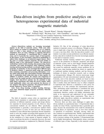
B. Image dataneural network, it can detect simple features, such as edges,at earlier layers, then later layers combine them to form somehigh level features. Since the pre-trained model is trainedon a huge amount of various types of images, the learnedfeatures have the ability to well characterize different types ofimages. Thus, the pre-trained model can be used as a featureextractor to extract features from images so that machinelearning methods could be further applied on the extractedfeatures to train the prediction model.In this work, we use a portion of VGG-16 [17] network asa feature extractor. As shown in Figure 2, VGG-16 consists offive convolutional blocks and two fully connected layers. Asmentioned above, the convolutional blocks (i.e. blue blocksin Figure 2) are used to learn the features that can wellcharacterize images, while the fully connected layers (i.e.red block in Figure 2) use the learned features to make theprediction. In this work, we keep the architecture and weightsof all the convolutional blocks of VGG-16 as feature extractorto extract features from SEM images of magnet samples. Thengradient boosting regressor is trained on the extracted featuresto make the predictions.Images of the magnet samples are taken after hot deformprocessing step using SEM technique. For each magnet sample, SEM images are taken at up to eight positions with threedifferent magnifications (i.e. 200, 1000, 30000) and twodifferent SEM modes (i.e. COMPO and SEI). In other words,there are at most 48 ( 8 3 2) SEM images for a magnetsample. Figure 3 (a) shows the two most common positionswhere SEM images are available in the dataset, the positionC00 is the center position of the magnet sample, while positionC10 is the position shifted along Z axis compared to positionC00. Figure 3 (b) shows an example of SEM image taken atC00 position with 1000 magnification and COMPO SEMmode.Fig. 3. (a) Illustration of the positions where SEM images are taken at amagnet sample. (b) An example of SEM image taken at C00 position with 1000 magnification and COMPO SEM mode.IV. M ETHODSA. Data preprocessingBecause the dataset is collected from experiments, thereare noise, missing values and outliers in the dataset. In orderto train an accurate prediction model, data preprocessing isnecessary.1) Data preprocessing for numerical data: For numericaldata, the data preprocessing, such as feature removal andoutlier detection, is mainly based on domain knowledge.Particularly, a four-step preprocessing method is applied onnumerical data to obtain the corresponding dataset. Numerical data includes the features representing composition and processing information of magnet samples.Since the dataset is relatively small, such large numberof features might lead to the curse of dimensionality.Thus, we remove features that are not related to magnetproperties (i.e. features that do not effect properties basedon domain knowledge) and features that are correlatedwith others (i.e. features that can be calculated based onother features). For example, manufacturing device nameis removed because it is not related to magnet properties,and the aspect ratio of a sample is removed since it iscorrelated with its width and length. Then we remove the data points without correspondingmagnet property.Fig. 2. Architecture of VGG16 pre-trained model. (bs. is the abbreviation ofbatch size)III. DATASETThis dataset is collected from experiments by Toyota MotorCorporation, Japan for magnet properties research, and itincludes numerical data and image data.A. Numerical dataAs shown in Figure 1, there are four processing steps (i.e.rapid cooling, molding, hot deform and heat treatment) toimprove the mechanical properties of a magnet sample. Thus,the numerical data mainly contains the processing informationof four processing steps, such as processing time, processingtemperature and pressure. The composition of the magnetsample is also included in the numerical data. In addition, atmost four magnet properties can be measured for a magnetsample. More specifically, Property No.1 (i.e. P1 Hcj andP1 Br) are measured after hot deform processing step, whileProperty No.2 (i.e. P2 Hcj and P2 Br) are measured after heattreatment processing step.808
an extensive grid search for optimization of hyperparametersto find the best hyperparameters. For instance, for gradientboosting regressor, we used a learning rate from [0.01, 0.1,0.5], number of estimators from [50,100,150,200] and maximum depth from [1, 3, 5, 10]. Similarly, for each pre-trainednetworks, different layers are tried as feature extractor to findthe best image representative for current application. Amongall of the combinations of regressors and feature extractors,the proposed models that use gradient boosting regressor andVGG-16 as feature extractor perform the best. In the nextsections, three types of models based on gradient boostingregressor and VGG-16 are proposed for each magnet property,which are numerical model, image model and combinationmodel.1) Numerical model: Numerical model (referred as Nummodel) takes numerical data as input and uses gradient boosting regressor to train the prediction model. More specifically,gradient boosting regressor with 0.1 learning rate, 100 estimators and maximum depth of 3 is used. The same parametersettings of gradient boosting regressor is used for both imagemodel and combination model, which are introduced later. Asmentioned in section 3, the number of features for differentmagnet properties are different. More specifically, the numberof input features of numerical model for Property No.1 andNo.2 are 40 and 43, respectively.In the experiments, the property of a magnet sample ismeasured multiple times, and the magnet property of thesame magnet sample might be slightly different due to themeasurement errors of the machine. Thus, we remove theoutliers (i.e., where the magnetic property is significantlydifferent from other same magnet sample), fill up themissing values with the average value from the samemagnet sample, and take the average value of the magnetproperty of the same magnet sample as the value of itsproperty. The range of different features are highly diverse, so werescale each feature individually to unit norm.After data preprocessing, there are 43 features left and theycan be categorized into four categories: Composition: The magnet sample consists of 9 chemicalelements. Dimension: There are 4 features describing the physicaldimension of the magnet sample before hot deformprocessing step. Phase: There are 18 features representing the informationof different phases in the rapid cooling processing step. Processing parameters: There are 12 features in totalrepresenting the processing parameters of the rest threeprocessing steps. More specifically, molding, hot deformand heat treatment processing steps include 4, 5 and 3features, respectively.Note that after data preprocessing, all the 43 features areavailable for predicting Property No.2, while only 40 featuresare available for predicting Property No.1, since Property No.1is measured before heat treatment processing step is appliedon the magnet sample.2) Data preprocessing for image data: As shown in Figure3 (b), the SEM image has label information at the bottom,which does not contain any structure information of the magnet sample. Thus, the bottom of each SEM image is cropped.Since the sizes of SEM images of different magnifications aredifferent, we then resize the SEM images to 224 224. Finally,the number of data points for each magnet property after datapreprocessing is listed in Table I. Fig. 4. The flowchart of the proposed image models.2) Image model: After analyzing the image data, we findthat using either three images (i.e. images of position C00with 3 magnifications and COMPO SEM mode) or six images(i.e. images of position C00 and C10 with 3 magnificationsand COMPO SEM mode) gives the best performance. Thus,two image models are proposed in this work. One imagemodel (referred as 3M model) takes three SEM images ofa magnet sample as input (i.e. images of position C00 with3 magnifications and COMPO SEM mode), while the otherimage model (referred as 6M model) takes six SEM imagesof a magnet sample as input (i.e. images of position C00and C10 with three magnifications and COMPO SEM mode,respectively). The flowchart of both image models are thesame, and it is shown in Figure 4, and it includes three steps: After image preprocessing, we use transfer learning technique to extract semantic image vectors from images.More specifically, we truncate VGG-16 by keeping all theTABLE IT HE NUMBER OF DATA POINTS FOR EACH MAGNET PROPERTY AFTERDATA PREPROCESSINGPropertyProperty No.1 - HcjProperty No.1 - BrProperty No.2 - HcjProperty No.2 - BrNumber of data points989810799B. Proposed modelsWe compare the performance of different combinations ofmachine learning methods such as gradient boosting, randomforest and support vector machine as regressors and pretrained networks such as VGG-16, VGG-19 [17] and ResNet[18] as feature extractors. For each regressor, we performed809
convolutional blocks (i.e. blue blocks in Figure 2), andfeed the preprocessed image into the truncated networkto get the output (i.e. 512 features maps) of the lastconvolutional block.However, the dimensionality of the output of the last convolutional block is too high, which might lead to the curseof dimensionality. Thus, we apply two methods to reducethe dimensionality. First, global average pooling [19] isapplied on each feature maps individual by computingthe average of entries’ values of each feature map. In thisway, we could convert these 512 feature maps to a 1-Dvector with 512 entries and it is the representation of theinput image. Since the image model takes multiple SEMimages as input, we compute such vector for each inputimage individually and concatenate them together intoone 1-D vector. However, the dimensionality of this 1-Dvector is still high compared to the number of features ofnumerical data, so Principal Component Analysis (PCA)[20] is applied to further reduce the dimension to 25. Inparticular, the summation of explained variance ratio ofthe selected principal components are around 91% and87% for 3M and 6M model, which implies the selectedprincipal components contain the enough information ofimages. In other words, by using transfer learning anddimensionality reduction techniques, we could use a 1-Dsemantic image vector with 25 entries to represent inputimages.Finally, gradient boosting regressor takes the semanticimage vectors as input to train the prediction model foreach magnet property.Fig. 5. The flowchart of the proposed combination models.and pearson correlation coefficient (R). The equations forcomputing three metrics are shown as below,M AE% (1) N(yi my )(ŷi mŷ )R i 1N22i 1 (yi my ) (ŷi mŷ )(2)where N is the total number of data points in the dataset ofcorresponding magnet property. yi and ŷi represent the groundtruth and predicted values, respectively. my and mŷ denote themean of the ground truth and predicted values, respectively. Inaddition, because the dataset is relatively small, 5-fold crossvalidation is implemented to evaluate performance of all theproposed models.B. Results analysis and data-driven insights3) Combination model: The combination model takes bothnumerical data and image data as input, and two combinationmodels are proposed in this work. The difference of the twocombination models is the number of input SEM images. Onecombination model (referred as 3NM model) takes three SEMimages of a magnet sample (i.e. images of position C00 with3 magnifications and COMPO SEM mode) and numericaldata as input, while the other combination model (referred as6NM model) takes six SEM images of a magnet sample (i.e.images of position C00 and C10 with three magnificationsand COMPO SEM mode, respectively) and numerical data asinput. The flowchart of combination model is shown in Figure5. More specifically, the method to compute the semanticimage vector from input images is the same as the imagemodel. Then the semantic image vector is concatenated withnumerical data, and they are fit to each magnet property usinggradient boosting regressor.V.N1 yi ŷi 100N i 1yiIn this section, the performance of the proposed modelsare evaluated and data-driven insights are discussed based onthe experimental results. The proposed models are trained foreach magnet property, and the results of 5-fold cross validationin terms of MAE% and R are shown in Table II and TableIII. From the results, we can observe that numerical modelcan already achieve a very high accuracy although it onlyuses numerical data as input. More specifically, the numericalmodel can get 3.56% and 2.20% MAE% for Property No.1Hcj and Br, respectively. For Property No.2 Hcj and Br,the numerical model can achieve 4.23% and 2.98% MAE%.Meanwhile, the results of Table III follows the same trend.TABLE IIP ERFORMANCE COMPARISON OF THE PROPOSED MODELS IN TERMS OFMAE%PropertyP1 HcjP1 BrP2 HcjP2 BrR ESULTS AND A. Experimental setting and error metricFigure 6 shows the parity plot of all the four magnetproperties based on numerical model. The plots show that mostof data points are distributed along the diagonal, which showsWe use two error metrics to evaluate the performance of theproposed models, which are mean absolute error rate (MAE%)810
TABLE IIIP ERFORMANCE COMPARISON OF THE PROPOSED MODELS IN TERMS OF RPropertyP1 HcjP1 BrP2 HcjP2 Mmodel0.780.570.810.393NMmodel0.930.630.960.55of 6M model for all the magnet properties is slightly betterthan that of 3M model. The reasons might be twofold: 1)The SEM technique would destroy the sample after takingthe image. So although the SEM image and magnet propertycould be collected from the samples with same compositionand processing parameters, there is no one-to-one mappingbetween SEM image and magnet property. In other words,the SEM images and corresponding magnet property arenot measured from exactly the same sample, which couldintroduce noise in the dataset. 2) There are six images (i.e.positions C00, C10 with three magnifications and COMPOSEM mode) available for each magnet sample. By taking moreSEM images as input, the model can learn more knowledgeabout structural information. Thus, the performance of 6Mmodels are better than that of 3M models. Another threeinsights could be found be analyzing and reasoning the resultsof the proposed image models:6NMmodel0.930.640.960.57that the proposed model can make accurate predictions. However, the variance of parity plot of Property Br is larger thanthat of Property Hcj. In addition, it is relatively straightforwardto retrieve importance scores for each feature after gradientboosting regressor is trained. In particular, feature importanceis calculated for a weak learner by the amount that each featuresplit point improves the performance measure. The featureimportance is then averaged across all of the weak learnerswithin the model. Figure 7 shows the feature importance foreach magnet property based on the numerical model. Insights (1): The four processing steps have differentpurposes. Rapid cooling is to make crystallization andcontrol the size of crystallization. Molding is to increasesample’s density. Hot deform aligns the orientation of thecrystal to get high property. Heat treatment smooths theunevenness of grain boundaries of sample’s structure toget high property. Thus the hot deform and heat treatmentprocessing steps are the crucial processing to enhance themechanical property of the magnet samples. In Figure 7,the features of hot deform and heat treatment processingsteps are found to be more important than other features,which matches the domain knowledge. Insights (2): From data mining point of view, it is important to retain a one-to-one mapping between model’sinput and output. Since SEM techniques could destroythe samples, it is important to change the experimantoperations order that the properties of samples should bemeasured before SEM images are analyzed.Insights (3): As shown in Figure 3 (a), the position C00is the center position of the magnet sample, while positionC10 is the position shifted along Z axis compared withposition C00. Since both positions are at the center areaof the magnet sample, the SEM images of the two positions might contain similar structural information. Thus,only slight performance improvement can be observedwhen we include more SEM images from position C10.The performance might be improved if more SEM imagesfrom other different sample areas are available.Insights (4): In addition, we can observe that the performance of the image models for Property Hcj are worsethan that of image models for Property Br. Interestingly,this might indicate that the structural information in theSEM images is more related to the property Br, but we arenot aware of any existing domain knowledge supportingor refuting this data-driven insight.The performance of 6NM model for all the magnet properties is slightly better that that of 3NM model, and thereasons for the improvement are the same as mentioned above.In addition, the performance of the combination model hasdifferent trends for Property Hcj and Br when compared withthat of the numerical model. As mentioned in insights (4), itappears that the structural information in the SEM images ismore informative for Property Br, so including SEM images inthe combination model leads to a performance improvementcompared to the numerical models for Property Br. On theother hand, since the performance of the image model is muchworse than that of numerical model for Property Hcj, addingSEM images in the combination model does not improvethe performance, but rather deteriorates the performance asit might confound the model.Fig. 6. The parity plots of each magnet property based on numerical model.(a) Property No.1 Hcj. (b) Property No.1 Br. (c) Property No.2 Hcj. (d)Property No.2 BrHowever, the performance of both image models is worsethan the corresponding numerical models, and the performance811
Fig. 8. The features importance for each magnet property based on 3NMmodel. (a) Property No.1 Hcj. (b) Property No.1 Br. (c) Property No.2 Hcj.(d) Property No.2 BrFig. 7. The features importance for each magnet property based on numericalmodel. (a) Property No.1 Hcj. (b) Property No.1 Br. (c) Property No.2 Hcj.(d) Property No.2 Br.Figures 8 and 9 show the feature importance for eachmagnet property based on 3NM and 6NM model, respectively.By comparing with Figure 7, we can observe that severalimage features turn out to be important to predict the magneticproperties. Howev
Data-driven insights from predictive analytics on heterogeneous experimental data of industrial magnetic materials Zijiang Yang , Tetsushi Watari†, Daisuke Ichigozaki†, Kei Morohoshi †, Yoshinori Suga , Wei-keng Liao , Alok Choudhary , and Ankit Agrawal Department of Electrical and Computer Engineering, Northwestern University †Toyota Motor Corporation, Japan