Transcription
Made available courtesy of the Royal Meteorological Society: http://www.rmets.org/***Reprinted with permission. No further reproduction is authorized without written permission from the Royal Meteorological Society.This version of the document is not the version of record. Figures and/or pictures may be missing from this format of the document.***INTERNATIONAL JOURNAL OF CLIMATOLOGY, VOL. 16, 195-2 1 1 (1996)RELATIONSHIPS BETWEEN GEOPOTENTIAL HEIGHTS ANDTEMPERATURE IN THE SOUTH-EASTERN US DUlUNG WINTERTIMEWARMING AND COOLING PERIODSPAUL A. KNAPP AND ZHI-YONG YINDepartment of Geography, Georgia State University, Atlanta, GA 30303-3083, USAReceived 27 October 1994Accepted 13 May 1995ABSTRACTThis paper discusses the relationship between geopotential heights and mean winter surface temperature and thecharacteristics of interannual variability in the south-eastem USA during cooling and warming periods from 1946 to 1992.Data fkom 83 Historical Climatology Network stations in 12 south-eastem states were examined. Factor analysis was used toseparate the southeast into three climatic regions. These regions were then matched with both 500 hPa and 700 hPa pressureheights during two periods: the 1946-1976 cooling period and the 1976-1992 warming period. The degree of associationbetween geopotential heights and surface temperature was greater during the cooling period than during the warming period.Possible influences may lie with differential temperature modification effects of the Gulf of Mexico and Atlantic Ocean, aswell as soil moisture variability. The amount of geopotential height variability, as measured by standard deviations, was alsocompared between the cooling and warming periods, and was significantly greater during the cooling period. This explains asimilar pattern in the surface temperature variability. A possible cause is the susceptibility of troughs to prolongation andamplification during cold winters. Both results suggest that not only is it difficult to determine the forcing mechanisms thatcause short-term variability, but that the influence of the forcing mechanisms may not be consistent between cooling andwarming periods as well.KEY WORDS: .south-eastem USA; winter temperature;temperature trends; geopotential heights; factor analysis; correlation; teleconnectionsINTRODUCTIONInterannual and interdecadal temperature variability is a source of great interest to humankind because of thepossible effects on human activities such as agriculture (Agee, 1980). Often, questions arise as to whether therecently observed variability is part of short- or long-term global or regional climate change, with itscommensurate effects on biospheric and socio-economic systems (Karl and Quayle, 1988). Additionally,considerable discussion exists in understanding the physical mechanisms that cause the changes. Finally,differences in the degree of interannual variability during warming and cooling periods suggest that the effects ofthese mechanisms may not be consistent.One of the most interesting features of interannual and interdecadal climatic variability is the fiequent andregional nature of the changes (Trenberth, 1990). Climate variations often are associated with changes in generalcirculation patterns (van Loon and Williams, 1976), with accompanying changes of opposite magnitude occuningconcurrently within the hemisphere (Stockton, 1990). During winter seasons in the eastern USA, for example,substantial cooling occurred between the early 1940s and 1980s (Agee, 1980), whereas winter temperaturedepartures in the western USA were predominately above average (Dewey and Heim, 1993). In the last decade,eastern USA winters have been characterized by substantial warming (Dewey and Heim, 1993).Cold and warm winters in regions of continental USA are often associated with anomalies of general circulationpatterns (van Loon and Williams, 1976), particularly the Pacific-North American (PNA), North AtlanticCCC 0899-8418/96/020195-170 1996 by the Royal Meteorological Society
196P. A. KNAPP AND Z.-Y. YINOscillation (NAO), and El Niiio-Southern Oscillation (ENSO) teleconnections (Rogers, 1984; Yamal and Leathers,1988; Redmond and Koch, 1991). These teleconnections are the linkage between atmospheric conditions over longdistances ( 2 2000 km), and the PNA teleconnection generally is viewed as the most important in influencingNorthern Hemisphere winters on the North American continent (Wallace and Gutzler, 1981; Simmons et al., 1983;Barnston and Livezey, 1987). The PNA teleconnection pattern is expressed as anomalies in either the 500 hPa or700 hPa geopotential height field, and can be represented as an index (Horel and Wallace, 1981; Wallace andGutzler, 1981; Yamal and Diaz, 1986).Variations in the PNA index represent periods of increased meridional or zonal flow, which in turn influencesurface temperatures in various regions. The classic PNA pattern (phase) is characterized by enhanced upper-leveltroughing in the north-east Pacific, ridging centred over the western Canada Rocky Mountain Cordillera, andtroughing over the eastern USA (Yarnal and Leathers, 1988). The opposite phase, the Reverse PNA (RP”), ischaracterized by the lowered ridge and filled troughs at the above locations. In extreme cases, the placement ofridges and troughs is the opposite of the PNA phase (Yamal and Leathers, 1988). The PNA index variessubstantially during the course of the year. Amplification of the long waves in the mid-troposphere (i.e. positivePNA index values for increased meridionality) is associated with above-normal temperatures in areas locatedbeneath the ridge (western USA) and below-normal temperatures in areas beneath the trough (eastern USA)(Leathers et al., 1991). Flattening of the long waves (negative PNA index) increases zonal flow, which bringsbelow-normal temperatures to the west and above-normal temperatures to the east. A PNA index value of zeroindicates minimal deviations from mean temperature conditions.Several studies have addressed specifically the relationship between upper-level circulation and wintertemperatures in the USA. Erickson (1984) investigated the relationship between area-weighted surfacetemperature in the USA and zonally averaged 700 hPa height. During warm winters in the USA, the 700 hPaheights generally have positive anomalies over subtropical and mid-latitudes and negative anomalies over highlatitudes. During cold winters in the USA, the opposite patterns were observed. Leathers et al. (1991)investigated the relationship between monthly temperature in the USA and upper-level flow patterns representedby a PNA index. They found that temperature is positively correlated with the PNA index in the eastem USAand is negatively correlated with the index in the west. Yamal and Leathers (1988) examined interdecadal andinterannual temperature variability in Pennsylvania between 1947 and 1982 and found that variations in PNAteleconnections explained 50 per cent of the wintertime variance. Klein and n i n e (1984) examined correlationsbetween concurrent winter mean monthly temperature anomalies at 109 stations and 700 hPa height anomaliesin the USA between 1948 and 1981. They determined that surface temperature at a given station may correlatehighly with pressure in two or more locations. The positive correlation centres tended to be located close to thereference station ( 1500 km),and the negative correlation centres were M e r away from the reference station.The highest positive correlations (r 0.80) were in the south-east. Skeeter (1990) calculated zonal andmeridional flow gradients in the 500 Wa height field. He found that the surface temperature in the north-westemand south-eastern USA were associated most strongly with upper-level flow conditions.Complicating the relationship between upper-level atmospheric conditions and surface temperature, is thetemporal and spatial inconsistency of interannual temperature variability during warm and cool periods. An oftenrepeated axiom with little verification is that temperature variability increases during cool periods and decreasesduring warm periods (van Loon and Williams, 1978). Several studies (e.g. van Loon and Williams, 1978; Karl,1988; Balling et al., 1990), however, have shown that there may be no systematic association between seasonalmean temperature and associated standard deviations. Conversely, Diaz and Quayle (1980) did find that, at least forthe winter mean temperature in the continental USA, cooler-more variable and warmer-less variable patternsexisted.The purpose of this paper is to address the relationship between interannual and interdecadal variability ofgeopotential heights and mean winter surface temperature in the south-eastern USA. In particular, we will examinetwo aspects of the relationship between geopotential heights and surface temperature that have been studied little.First, we will explore how the association between 500 hPa and 700 hPa heights and surface temperature variesbetween warming and cooling periods. Second, we will examine the degree of temporal variability of geopotentialheights during warming and cooling periods.
WINTER TEMPERATURES IN SOUTH-EASTERN USAN Station NumberSSWJO&197’Figure 1. Location of Historical Climatology Network station sites used in this studySTUDY AREAThe study area includes 12 States in the south-eastern USA: Alabama, Arkansas, Florida, Georgia, Kentucky,Louisiana, Mississippi, North Carolina, South Carolina, Tennessee, Virginia, and West Virginia. The study area islocated between 24’30” to 40’36’N and 75’27‘W to 94’37’W. The climate is characterized by hot, humidsummers and mild winters (Trewartha and Horn, 1980). Mean January temperatures range from 0 C in themountains of West Virginia to above 20 C in the Florida Keys.DATA AND METHODSTemperature dataTemperature data were acquired from the United States Historical Climatology Network (HCN) serialtemperature data set (Karl et al., 1990). These mean temperature data have been adjusted fully for urbanizationeffects, station moves, instrument changes, and time-of-observation biases. The original data set was pared fromthe 48 coterminous States to the 12 south-eastem States in the study area. The south-eastern data set included 276stations, which was further reduced to 83 stations (Figure 1). We reduced the data set by including only stationswith a HCN consistency ranking within the top 30 per cent of all stations. The ranking of a station is based on datafor its 20 nearest neighbouring stations during the last 40 years (Karl et al., 1990). The number of stationsrepresented in each State ranged from three (Alabama) to 10 (Georgia and South Carolina).The temperature data used were mean seasonal values beginning in 1946 and continuing through to 1992.Winter temperature data were represented by December (of the previous year), January, and February.
198P. A. KNAPP AND Z.-Y. YIN500 hPa and 700 hPa pressure height dataBoth 500 hPa, beginning in 1946, and 700 hPa height data, beginning in 1947, were represented in seasonalformat identical to temperature. The pressure data were provided by the National Center for Atmospheric Researchfrom the National Meteorological Center data set (Jenne, 1975). The 700 hPa heights were observed twice a day(0000 and 1200 UTC). For each month, the 0000 and 1200 UTC monthly observations were averaged. The500 hPa data were more complicated. During the period 1946 to March 1955, observations were taken only at1200 UTC. During April 1955 to May 1957, observations were taken at 0300 and 1500 UTC. Afterward,observations were taken at 0000 and 1200 UTC, the same as the 700 hPa data. To avoid errors associated withchanging observation times, we used only the observations at 1200 UTC from 1946 to March 1955 and fiom June1957 through to 1992. From April 1955 to May 1957, we used the observations at 1500 UTC. Data for grid points,separated by 5" latitude and 5" longitude, ranged from 20"N to 60"N, and from 70"W to 125"W (Figure 2).Sea-surface temperature dataSea-surface temperature (SST)data were provided by Scripps Institution of Oceanography, and were a subset ofthe Comprehensive Ocean-Atmosphere Data Set (COADS). The data were presented as monthly means from shipobservations based on 2" x 2" grid boxes. The length of record was from January 1946 to December 1992. Wesummarized the data seasonally, beginning in December 1946 (for winter 1947) through to 1992. We used SSTdata between 20"N to 40"W and 60"W to 96"W (Figure 3). We recognize that the reliability of SST is relatively lowbecause the number of observations in each month was different, especially during the earlier years.RegionsWe defined our climatic regions by performing factor analysis on the 83 south-east HCN stations using meanannual temperature data. Annual temperature data were used because they give the best average approximation ofthe regional boundaries. Three factors were retained based on two criteria: cumulative eigenvalues exceeding 80per cent of the total variance in the matrix (in this instance, the three factors represented 87.2 per cent) andidentifying the point of inflection (break in slope) on the scree plot (Zar, 1984). The three factors were thenorthogonally rotated using a VARIMAX rotation (SAS, 1988). The highest factor loading for each station was thenused to place a station in a region (Figure 4). Region 1 represents 39 stations where the highest loading was on thefirst factor. Region 2 represents 27 stations with their highest loadings on the second factor, and region 3 marks 17stations with their highest loadings on factor three. Regional temperatures were then calculated as the average forall stations within each region.MethodsPearson product-moment correlation analyses were performed for each region between winter temperature andboth 500 hPa and 700 hPa pressure heights for each grid-point. Correlation coefficients were mapped usingSURFER@ to show spatial patterns of the correlation field. Similarly, Pearson product-moment correlation analyseswere performed between winter surface temperature and winter SST. Likewise, correlation coefficients weremapped with SURFER@. For each region, we plotted temperature and pressure height of the grid-point with thehighest correlation coefficient during the length of record. These plots allowed us to separate the temperaturerecord into cooling and warming periods based on an inflection point. We selected five grid points (both 500 hPaand 700 hPa) that had the highest correlations between temperature and pressure heights for each region. Theconsistency of the relationship between temperature and pressure height was then examined using a matched-pairsStudent's t-test on correlation coefficients during different periods. If the mean correlation coefficients for twoperiods (i.e. warming versus cooling) are statistically different, then the relationship between temperature andpressure heights is inconsistent between wanning and cooling periods. Because the cooling period is almost twicethe length of the warming period, potentially biasing the selection of grid-points, we also selected five grid-points(both 500 hPa and 700 hPa) that had the highest correlations between temperature and pressure heights for each
WINTER TEMPERATURES IN SOUTH-EASTERN USA199Figure 2. Locations of 5" latitude by 5" longitude intersections for 500 hPa and 700 hPa geopotential height dataregion for both the cooling period and warming period. We then ran an independent Student's t test comparingcorrelation coefficients between time periods. Finally, we also performed similar analyses on the associationbetween SST and surface temperature using the five grid-points with the highest correlations.In comparing the interannual variability of pressure heights during warming and cooling periods, we determinedthe standard deviation of 500 hPa and 700 hPa height pressure at the same grid points as above (i.e. those with thefive highest correlations) and again performed a matched-pairs Student's t test. Statistically different standarddeviations of pressure heights between warming and cooling periods would suggest that the amount of interannualvariability is also inconsistent.Figure 3. Shaded area represents region From where sea-surface temperature data were used in this study
200P. A. KNAPP AND Z.-Y. YINFigure 4. Boundaries of the three defined climatic study regionsRESULTSCorrelation coefficients between temperature and pressure for each region show distinct spatial patterns, and wereconsistent between 500 hPa and 700 hPa heights (Figures 5 and 6). The highest correlations for each region arecentred on the southeast coast from the Florida Panhandle to Chesapeake Bay, as opposed to being centred directlyover the specific regions. For region 1 and region 2, maximum correlation coefficients were below 0.90, whereasfor region 3 maximum r values were greater than 0.90. Correlation coefficients decreased substantially west of93"W to approximately 105"W. From the Rocky Mountains north-westward, correlation coefficients show anincreasingly negative relationship, peaking between - 0.50 and - 0.60 in central Alberta.The temperature record for all three regions show a distinct inflection point, from a cooling trend from 1946through to 1975 to a warming trend from 1976 through to 1992 (Figure 7 and 8). Mean correlation coefficientsbetween temperature and both 500 hPa and 700 hPa heights for selected grid points are statistically greater(p O.O5) during the cooling period than that during the warming period (Tables I and 11). These correlationcoefficients suggest that during periods of cooling, the linear relationship between temperature and pressureheights is stronger than during warming periods (Figures 7 and 8). Additionally, comparisons between Tables I andI1 show that the selection of grid-points in this study is not statistically biased by the differential length of warmingand cooling periods. Although the pressure height grids with the high correlation coefficients shifted in the laterwarming period, this did not affect the results of the statistical test.Standard deviations of both 500 hPa and 700 hPa pressure heights for selected grid points are significantlygreater (p 0.001) during the 1947-1975 cooling period than during the 1976-1992 warming period (Tables I11and IV). A similar decrease in standard deviation is also found for the surface temperature (Table V). Greaterstandard deviations suggest that during the cooling period, there is greater interannual variability in pressureheights and surface temperature. The initial sample size for pressure height standard deviation values was 30 (3regions x 2 geopotential heights x 5 grid points per region), but was subsequently reduced to 17 because we didnot double count 13 grid-point observations that were included in more than one region.
WINTER TEMPERATURES IN SOUTH-EASTERN USA20 1Figure 5. Correlation coefficientsbetween mean winter temperature and 500 Wa pressure heights for (a) region 1, (b) region 2, and (c) region 3Correlation coefficients between surface and sea-surface temperatures were typically highest ( 0 . 5 4 6 ) on thecoastlines for both the Gulf of Mexico and Atlantic Ocean (Figure 9). Associations generally decreased south ofthe Gulf of Mexico and east of the Atlantic Ocean shorelines. Little spatial variation in correlation coefficientsexisted between the three regions. Correlations during the cooling period were again significantly greater(p O.OOOl) than during the warming period (Table VI), suggesting that the influence of SSTs on surfacetemperatures is inconsistent.
202P. A. KNAPP AND Z.-Y. YMFigure 6. Correlation coefficients between mean winter temperature and 700 hPa pressure heights for (a) region 1, (b) region 2. and (c) region 3DISCUSSIONOur results show a high degree of association between upper level pressure heights and surface temperature. Theseresults are in close agreement to other similar studies (e.g. Klein and Kline, 1984), and further confirm that upperlevel conditions have a strong influence on surface temperatures. What we found of great interest, however, wasthat this association was expressed stronger during the 1946-1975 cooling period than during the 19761992warming period. Our interest in these transition periods as opposed to warm and cool periods was based on the
203WINTER TEMPERATURES IN SOUTH-EASTERN USA500 MB WINTER REBION 1.58m2.0.- .bT6660Moo0.0 '11040low100I07010801890YEPR515012.010.0.z1".f6.0. .4.0. . . -s600ss-5100.r-soy-3I!11.0,-5750500 MB WINTER REGION 3.P.t-194O1-Figure 7. Time series of mean winter temperatures and 500 hPa pressure heights, 1946-1992understanding that many positive feedback mechanisms occur during either warming or cooling periods, such asaltered baroclinicity (Dickson and Namias, 1976), which enhances these trends. Further, as Stockton (1 990) hasargued, climatic variability on the order of 10 to 100 years is of greatest importance to human activities because thevariability is typically regional in nature and affects all activities dependent upon temperature, including agricultureand municipal planning.
204P. A. KNAPP AND Z.-Y. YM0.0 ,3140I700 MB WINTER REGION 2.b,.34P6.0 .-i"!-xm-4.0 .2.0I '-I19401050ls6u1970lgeo1990#xx)EM314031203100 ih s3MoJ. 300619401950lsao19701-1980zgo2OOoYEARFigure 8. Time series of mean winter temperatures and 700 hPa pressure heights, 1947-1992One explanation of stronger association during cooling periods may rest with the differential temperaturemodification effects of the Gulf of Mexico and the Atlantic Ocean. During periods of negative pressure heightanomalies in the south-east (enhanced troughing that characterized the cooling period), the prevailing atmospheredynamics involved the advection of cooler drier air from interior North America and a strong PNA teleconnection
205WINTER TEMPERATURES IN SOUTH-EASTERN USATable 1. Correlation between winter temperature and pressure heights of 500 hPa and700 Ma levels for selected grid-points, and matched-pairs Student’s t tests on correlationcoefficients during 1946-1 975 and 1976-1 992 Geopotentialheight p a )500With temperature ofRegion 1Region 2Region 3700Region 1Region 2Region 1540.831870.754780.634980.795510.802160.8 s Student’s t test500 and 700 hPa500 hPa700 hPaNMean 23150.05713.65150.0026(Dickson and Namias, 1976; Klein and Kline, 1984). The north-westerly flow aloft tends to minimize the influenceof moderating air flows, particularly the south-westerly flow from the Gulf of Mexico. The jet-stream trajectoriesshift southward and increase cyclonic activity in the south-east. During such times, strong cold waves may bringArctic air to the Florida Peninsula, which has caused serious damage to the citrus trees (Rohli and Rogers, 1993).With the passage of each cold front, surface temperatures decrease rapidly because of the advection of cold airbrought by the north-westerly flows as well as radiational cooling. The cold, dry weather behind the cold frontreduces the frequency of events, such as persistent fog and low stratus clouds, that have been shown to lowercorrelations between surface temperature and geopotential heights (Klein and Kline, 1984).Unlike the relatively dynamic forcing mechanisms dominant during the cooling period, surface temperatures inthe south-east may be affected by several forcing mechanisms during the warming period. During periods of
206!I A. KNAPP AND 2.-Y. Y MTable 11. Correlation between winter temperature and pressure heights of 500 hPa and 700 hPa levels forselected grid-points, and independent Student’s t tests for correlation coefficients during 1946-1975 and1976-1 992Geopotentialheight (hpa)500With temperatureOfRegion 1Region 2Region 3700Region 1Region 2Region 3Grid-points Years 9030W7035W7530w7535W8030W8035Grid-points Years 9229 10.941 46180474800.849300.886600463520.809250-817340.8 15050-815700.8 0.802160.819910.8 930.88640Independent Student’s t test500 and 700 hPa500 hPa700 hPaNMean differenceta300.03744.067 10 0001150.02862.054604494150.0462341450.0007positive pressure height anomalies (decreased troughing that characterized the warming period) the polar front jetis displaced northward, and there is a substantially stronger south-westerly flow into the south-east. Consequently,there is an increase in the frequency of the warm, maritime air m s e s that originate in the Gulf of Mexico(Dickson and Namias, 1976; Leathers el al., 1991). In this instance, warming temperatures in the southeast are notonly influenced by south-westerly flow, but would be modified by SSTs that lag with upper level pressure heights.Lanzante (1984), for example, determined that 700 hPa heights significantly led Atlantic SSTs by one to twomonths from January to March.Correlations between SSTs and surface temperatures during the cooling and warming periods support this notionof the complicating effects of the ocean. Similar to the relationship between surface temperatures and pressureheights, there is a weaker association between SSTs and surface temperature during the warming period than the
207WINTER TEMPERATURES IN SOUTH-EASTERN USATable 111. Means and standard deviations of 500 hPa and 700 hPa heights for selected grid-points during1946-1975 and 1976-1992Geopotentialheight p a W85N35W80N30W75N30W85N305664.4056574455 5.423053.013050.672968.613048.4331 17.123 121.6131 .38963 130.18997128.69833026.5242442545447324.59816424.3 2968.533047.973 116.923 0634.929093 1.8989923.7 I45725.7055026.139592 1.9915822.771 1424.888342 1.6954317.7744417.2556917.85444Table N Matched-pairs Student’s t test on standard deviations of pressureheights during 1946-1975 and 1976-1992 for selected grid-pointsNMean differencetU500 and700 hPa500 hPa700 hPa175.73248.70390.000 196.10985.721685.30796.89790.00020.0004Table V Means and standard deviations of surface temperature during 1946-1975 and1976-1 992I-1946-19751976-1992LocationMeanSDMeanSDRegion 1Region 2Region 12.78961.51311.51851.3007cooling period (Table VI). Apparently, strong dynamic forcing mechanisms also caused SSTs along the south-eastcoast to change, synchronized with the variations in the surface temperature during the cooling period. During thewarming period, a plausible explanation may involve recent work that has refocused on the long-term memory ofoceans to store heat and to modifL the effect of surface heating (Watts and Morantine, 1991, 1993; Kellogg, 1993).These studies have suggested that oceanic circulation changes have the potential to redistribute sensible heat
208I? A. KNAPP AND Z.-Y.YINTable VI.Correlation coefficients between surface temperature andsea-surface temperature for selected grid-points during 1946-1975and 1976-1992With T of:Grids1946-19751976-1992Region 230-607580.781550.631230.601 150.490660.65235044509*Region 2W78N34W88N28W94N22W94N26W96N280.753700.7203 *0.45697*Region 3W82N30W94N22W84N24W94N26W80N2804337 50.510560.53833* Not significant at the 0.05 level.energy and influence surface temperatures (Watts and Morantine, 1993). Hence, the reduced association betweenupper level pressure heights and surface temperatures during the 1976-1992 period may have been affected by thestored thermal energy coupled with the more northern position of the polar front jet.Additional mechanisms may complicate the association between upper level pressure heights and surfacetemperature. Soil moisture variability has been shown to create surface temperature anomalies throughmodifications of the Bowen ratio (sensiblehatent heating ratio) (Walsh et al., 1985), although having little impacton the upper atmosphere (Yang et al., 1994). Additionally, abnormally moist soil may be coupled with increasedhaziness, relative humidity, and
Data fkom 83 Historical Climatology Network stations in 12 south-eastem states were examined. Factor analysis was used to . teleconnections (Rogers, 1984; Yamal and Leathers, 1988; Redmond and Koch, 1991). These teleconnections are the linkage between atmospheric conditions over long . and the negative correlation centres were Mer away from .