WIXLIB

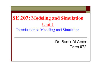
JOURNAL OF COMPUTERS, VOL. 8, NO. 4, APRIL 2013λ gT2th ( kh ) 2πc λT gT2πth (2π2gTth (2πλ2πλh) ,1029(12)h) .(13)According to the relationship of velocity potential andvelocity, the motion velocity of any seawater particlecould be obtained in (14) and (15). According to (11) (13), the motion trajectory of seawater particle wasobtained in (16) and simplified in (17).u gka ch[ k ( h z )] sin( kx ωt ) ,ch ( kh )ωw {a(14)gka sh[ k ( h z )] cos( kx ωt ) ,ch ( kh )ω( x x0 )2ch[ k ( h z0 )]sh( kh) } {2a( z z0 )density was set to be 1.225kg/m3 in the operationenvironment, while the gravity was considered.(15)2sh[ k ( h z0 )]sh ( kh )}kz222( x x0 ) ( z z0 ) ( ae ) .02 1,(16)(17)Eq. (16) represented that the motion trajectory ofseawater particle for linear wave was a circle.Furthermore, its radius decreased rapidly while waterdepth (-z0) increasing. When it came to a certain depth,the motion disappeared. This properties were consideredin C program of UDF.Figure1. Schematic diagram of numerical water areaThe velocity inlet was on the left of the model, whilethe velocity outlet was on the right. At initial time, thecalculation domain was initialized, and the water volumefractions above and below the free surface were set to 0and 1, respectively. The direction of current velocity wasset perpendicular to the left inlet boundary. The topboundary was set to pressure inlet, whose direction wasperpendicular. The bottom of the domain was set to wall.The cleft of oil tank was set to the boundary condition ofinterior, and the other parts were set to the boundarycondition of wall. PISO algorithm based on pressuresolution was adopted to solve the coupling problem ofpressure and velocity under unsteady states, and was usedby some researchers for fire and explosion prediction [16].The time step of numerical calculation was 0.005s. Theflow chart for FLUENT simulation is shown in Fig. 2.GAMBIT mesh initial definegrid checkNoYesdefine solver as unsteadychoose multiphase model asVOFIII. COMPUTER SIMULATIONSome assumptions were made for the model: theimpact of ship shaking on the oil level in tank was notconsidered; the three-phase flow of oil, water and gas wasnot compressible and not inter-miscible; the oil spillprocess was adiabatic and the three phases wereisothermal flow, regardless of thermal exchange amongdifferent phases; there was no broken ice in the seawaters.One side of ship was cracked by some external forceand the cleft was in the opposite direction of oceancurrent. The oil tank was rectangular and it contained thediesel of 985kg/m3. The upper part of calculation areawas atmosphere, while the lower part was water with icesheet covered on the right surface, as shown in Fig. 1.The grids of the whole calculation domain wererectangular.The two-dimension, unsteady and separated implicitsolver was adopted. The number of phases in VOF modelwas set to 3, where air was the basic phase, water was thesecond phase and oil was the third phase. The GeoReconstruct was used as the free surface reconstructionformat. The reference pressure was set to be the standardatmospheric pressure and the value of working fluid 2013 ACADEMY PUBLISHERinput ice water and oilpropertiesset phase number as 3use UDF to define boundariesadjust k, εchosse solver as PISOinitializeadapt regionsiteratecheck convergenceNoYesoutput dataFigure 2. Flow chart for software simulationThe wave was one of important ocean motion formsand could appear from ocean surface to interior. In orderto simulate damaged ship oil spill in Arctic shipping routemore precisely, the oil motion in ice water with theinteraction of wave and current was simulated, taking

1030JOURNAL OF COMPUTERS, VOL. 8, NO. 4, APRIL 2013linear simple harmonic wave for example. The propertiesof oil and seawater were given below: the oil kinematicsviscosity coefficient and surface tension coefficient wereυ0 1.053 10-5m2/s and σ0 200μN/cm, respectively. Theseawater density was ρw 1025kg/m2, and kinematicsviscosity coefficient was υw 1.7 10-6m2/s.As artificial viscosity method was insensitive to thefrequency or wavelength of incoming wave, and wasmore effective to adsorb incoming waves with differentfrequency or wavelength, this method was a good waveadsorbing method for establishing a general numericalwave flume. Therefore, the artificial viscosity methodwas adopted in order to prevent the interference of wavereflection in flume. The essential of this method was toadd damping term in the wave adsorption section. Inaddition, the length of wave adsorption section should beone time of incoming wavelength, as the effects on waveadsorption was related to the length of wave adsorptionsection.The interaction process of ocean wave and current canbe separated to three stages. The wave and current existindependently at the first stage, mix at the second stageand form steady union at the third stage. Therefore, thevalue of velocity was superimposed by the velocities ofwave and current:u u0 gka ch[ k ( h z )] sin( kx ω t ) .ch( kh )ωFigure 4. Wave profileIV. SIMULATION VALIDATIONThe trajectory of the oil spilled from the oil tank wasshown in Fig. 5 to Fig. 9, where the yellow, light blue anddark blue areas stood for the air, water and oil,respectively. In each figure, picture (a) stood for thecondition of oil spill site closer to the ice sheet, whilepicture (b) was for the far site and picture (c) was for thecondition of oil spill site closer to the ice sheet withnulclear wave.a(18)The symbol of u0 represented the seawater currentvelocity. When wave and current coexisted, the energyconservation of them should be considered for waveadsorption. In order to achieve energy conservation,outflow boundary conditions were set corresponding toinflow boundary conditions besides wave adsorptionsection.The flume model with wave source is illustrated in Fig.3. The wave point source of vertical distribution is set onthe left of flume, while damping wave adsorption sectionis set on the right. The potential flow theory is suitablefor the whole flow field. The damping coefficient of μ iszero on the surface facing waves in wave adsorptionsection, which make potential function continuousvariation. Then μ is the linear function of x. S1 stands forthe right and left boundaries. W stands for the bottomboundary of flume. The up free surface is pressureboundary. S1 and S2 are computational domains, amongwhich S1 is damping wave adsorption.Figure 3. Wave flume modelThe source term, the initial conditions and boundaryconditionsaredefinedbythemacroofDEFINE SOURCE(my source x, c, t, dS, eqn),DEFINE INIT (my init function, domain), DEFINE 2013 ACADEMY PUBLISHERPROFILE (x velocity in, thread, index), DEFINEPROFILE (y velocity in, thread, index) and DEFINEPROFILE (voffactor, thread, index), respectively ，which was shown in Appendix A. The result ofsimulation is shown in Fig. 4.bcFigure 5. Distribution of oil-water-air at time of 10sFor the different liquid levels in and out of oil tank atinitial time, the oil injected through the cleft and formedjet or plume into the external seawater, and was quicklybroken up to the droplets by the coming flow. As thedensity of oil was less than that of water, the oil floatedupwards in the form of droplets group by the waterbuoyancy. At the mean time, the oil group inclined to thespreading direction of ocean currents with the carryingaction of coming flow. When the oil spill site was closeto the ice sheet, the rising oil droplets would beintercepted by the edge of ice and adhere to the lowersurface of ice, after the oil reached the ice sheet as shownin Figure 5a. When the oil spill site was far from the icesheet, the oil would not reach the ice sheet within a shorttime and could easily rise to the sea surface without any

JOURNAL OF COMPUTERS, VOL. 8, NO. 4, APRIL 2013barrier, as shown in Fig. 5b. The obvious water particlescircle motion appeared to the inverse direction of wavetransmission. Contrary to this phenomenon, the violentextent of motion decreased along the direction of wavetransmission near surface, as shown in Fig. 5c. The wavepromoted the dispertion and transport of the oil.With the fluid level in oil tank falling gradually overtime, the pressure difference inside and outside changedlower and lower. This led to the amount and velocity ofoil spill declining gradually. Thus the concentration of oilnear the tank cleft decreased significantly. At this time,the oil floated gradually along the wake flow trajectory ofprevious oil droplets, with the action of sea current andwater buoyancy. When the oil spill reached sea surface,oil became to expand in the form of oil film with theaction of gravity and surface tension. And the thicknessof oil film became less, along with the oil expandingscope increasing.At the condition of oil spill site near to the ice sheet,the spreading and diffusion of oil film was influenced bythe lower surface of ice. The diffusion velocity was lowerbecause of the friction force action. Thus the diffusiondistance of oil film was significantly less than that on thefree sea surface at the same temperature. Thisphenomenon was shown in Fig. 6.ab1031surface reduced or even disappeared finally; Thisphenomenon would have a significant impact on theArctic environment; The presence of oil would increasethe probability of ice melting and shorten the meltingtime of ice sheets; The sunlight absorption by ice sheetwith oil was 30% higher than the regular ice sheet, andthe melting time would be advanced by about 7 to 21days.Fig.7. Velocity vector near the ice sheet edge at 20sWith time passing by, some oil could be scoured byseawater to form various sizes of droplets and dispersedin different depths of water. The large size dropletsfloated gradually and reaggregated with oil film on thesea surface, while the small size ones suspended in waterfor a long period of time. As the temperature of Arcticareas was lower than others, the viscous resistancebetween oil and water was relatively high, which led tothe lower velocity of oil spills spreading and moving.Moreover, since the water temperature was low and evenclose to zero, the discretization of oil spill was notobvious in ice waters, while this action occurredobviously in a fully open free surface of no ice waters.Thus the thick oil film was easy to form on the icy seasurface, as shown in Fig. 8.acbFigure 6. Distribution of oil-water-air at time of 20sIn addition, the spreading oil film could be blocked byice and easily formed the vortex at the edge of ice sheet.Then some oil would be entrained to the ice sheet surfaceand continued to spread and diffuse by the action ofsubsequent flow, as shown in Fig. 7. And Fig. 7 was forthe velocity vector distribution under the conditions of oilspill site closer to the ice sheet. This simulation result wasvery similar to the early phenomenon of the oil fieldexperiment made in the Canadian arctic high latitudes byComfort et al. [17]. That is: when the oil spill site wasclose to the ice sheet, some oil would transport onto theice surface and would be absorbed by the snow or carriedaway by wind over time; As a result, the oil on the ice 2013 ACADEMY PUBLISHERcFigure 8. Distribution of oil-water-air at time of 40sIn addition, besides the characteristics mentionedabove, there were other obvious differences between theoil film close to and far from the ice sheet. As shown inFig. 8a, the oil film which was generated from the oilspill site close to the ice would float beneath the ice sheet.And for the friction action of the lower ice surface, the

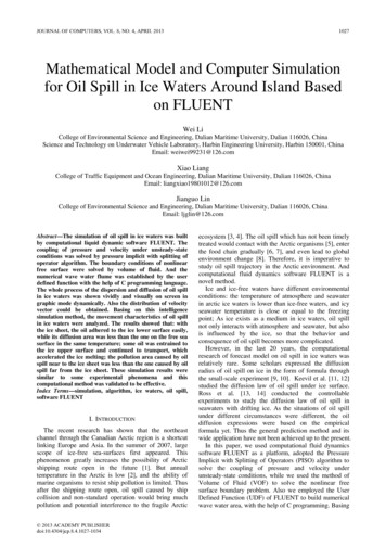
1032JOURNAL OF COMPUTERS, VOL. 8, NO. 4, APRIL 2013transport velocity of oil film was lower than that on freewater surface. Therefore, its oil film area was less thanthe one generated from the oil spill site far from the icesheet.As illustrated in Fig. 9a, the oil droplets below waterwould float to the lower ice surface and gatheredgradually for barrier of ice sheet. This computationalsimulation was the same to the experiment results, whichwas obtained by Greene [18]. In his laboratoryexperiment, the icy water tank was applied to research themovement of oil spill beneath the ice sheet surface, andthe phenomenon of a certain thickness oil film formingunder the ice sheet was observed. At this time, becausethe pressure difference between internal and external ofoil tank decreased to 0, the oil in tank would not spill anymore, while the spilled oil transported and diffusedgradually in the form of oil film with the action of seawater current.At the condition of oil spill site far from ice sheet, asshown in Fig. 9b, the oil was blocked by the edge of icesheet after it reached sea surface. This simulation wassimilar to the phenomenon shown in Fig. 6a: some oilwas entrained to the ice surface by the action of vortexand would disappear over time for weathering. On theother hand, most of oil would transport toward the lowerice sheet surface and diffused downstream with sea water.Because this part of oil would not contact with air andthere was no weathering action here, it required people toadopt remedial measures to clean up. It could be drawnfrom Fig. 6b that oil amount spilling out of the tank wasmore than that in Fig. 6a. Thus the oil film in Fig. 6b wasfar thicker than that in Fig. 6a and it was easier to recover.amathematics simulation method could simulate the oilspill in icy waters with less errors.Figure 10. Residuals of continuity, x, y velocity, k and εV. CONCLUSIONSIn this paper, we proposed a computational method tosimulate the trajectory of oil spill in icewaters aroundisland. The computational liquid dynamic softwareFLUENT was adopted. The numerical water flume wasestablished by UDF of FLUENT with the help of Cprogram language. The PISO algorithm was used to solvethe coupling of pressure and velocity under unsteadystate conditions, while the method of VOF was used tosolve the nonlinear free surface boundary problem. Onthis basis, the model of oil spill influenced by sea current ,ice and wave was researched. The results showed that thesimulation of oil spill was similar to some previouslaboratory experiments phenomena, which indicated thatour proposed computational technique based on softwareFLUENT was an effective method for oil spill simulationin ice waters.APPENDIX A PROGRAM IMPLEMENTATION OF MACRObcFigure 9. Distribution of oil-water-air at time of 100sIn this mathematics and computational simulationprocess, the residuals of x velocity, y velocity andcontinuity were monitored simultaneously and shown inFig. 10. The residuals of y velocity less than 1 10-5, theresiduals of x velocity less than 1 10-3 and the residualsof continuity less than 1 10-3 indicated that this 2013 ACADEMY PUBLISHERDEFINE PROFILE(x velocity in,thread,index){real x[ND ND];real y;face t f;real t;real u;t RP Get Real("flow-time");begin f loop(f,thread){F CENTROID(x,f,thread);y x[1];if(y (a*cos(w*t)))u a*w*cosh(k*(y h))*cos(-w*t)/sinh(k*h) ux;/*u a*w*cosh(k*(y h))*cos(w*t)/sinh(k*h) ux;*/else u 0.0;F PROFILE(f,thread,index) u;}end f loop(f,thread)}DEFINE PROFILE(voffactor,thread,index){

JOURNAL OF COMPUTERS, VOL. 8, NO. 4, APRIL 2013real x[ND ND];real y;face t f;real t;t RP Get Real("flow-time");begin f loop(f,thread){F CENTROID(x,f,thread);y x[1];if(y (a*cos(w*t)))F PROFILE(f,thread,index) 1.0;else F PROFILE(f,thread,index) 0.0;}end f loop(f,thread)}DEFINE SOURCE(my source x,c,t,dS,eqn){real x[ND ND];real mu,source;C CENTROID(x,c,t);mu 10*x[0];source -mu*C U(c,t);dS[eqn] -mu;return source;}DEFINE INIT(my init function, domain){cell t c;Thread *t;real x[ND ND];thread loop c (t,domain){begin c loop all (c,t){C CENTROID(x,c,t);/*if (x[1] 0)*/C U(c,t) 0.0;C V(c,t) 0.0;}end c loop all (c,t)}}ACKNOWLEDGMENTThe authors wish to thank the National Natural ScienceFoundation of China (Grant No. 51208070), Special Fundfor Marine Scientific Research in the Public Interest(201005010), China Postdoctoral Science Foundation(20110491519) and Fundamental Research Funds for theCentral Universities of China (2011QN052, 2012QN057).This work was supported in part by a grant from thesefunds.REFERENCES[1] D. Pietri, A. B. Soule, J. Kershner, P. Soles and M.Sullivan, “The Arctic shipping and environmentalmanagement agreement: a regime for marine pollution,”Coastal Manage. vol. 36, pp. 508–523, 2008. 2013 ACADEMY PUBLISHER1033[2] S. Løset, K. Shkhinek, O. T. Gudmestad, P. Strass, E.Michalenko and R. Frederking, et al., “Comparison of thephysical environment of some Arctic seas,” Cold Reg. Sci.Technol. vol. 29, pp. 201–214, 1999.[3] S. E Magnus, E. Øyvind, B. Øyvind, W. B. Odd, H. E.Ingrid and R. Kjell et al., “Prevention of oil spill fromshipping by modeling of dynamic risk,” Mar. Pollut. Bull.vol. 54, pp. 1619–1633, 2007.[4] J. Henrik, C. S. Rolf, A. Endre, A. Endre and S. Steinar,“The Arctic is no longer put on ice: Evaluation of Polarcod as a monitoring species of oil pollution in cold water,”Mar. Pollut. Bull. vol. 60, pp. 390–395, 2010.[5] L. G. Faksness and P.J. Brandvik, “Distribution of watersolube components from oil encapsulated in Arctic sea ice:Summary of three filed seasons,” Cold Regions Sci.Technol. vol. 54, pp. 106–114, 2008.[6] M. L. Hannam, S. D. Bamber, A. J. Moody, T. S.Galloway and M. B Jones, “Immunotoxicity and oxidativestress in the Arctic scallop Chlamys islandica: Effects ofacute oil exposure,” Ecotoxicol. Environ. Saf. vol. 73, pp.1440–1448, 2010.[7] P. H. Henry, A preliminary assessment of threats to arcticmarine mammals and their conservation in the comingdecades, Mar. Poli. vol. 33, pp. 77–82, 2009.[8] V. F. Krapivin and G. W. Phillips, Application of a globalmodel to the study of Arctic basin pollution: radionuclides,heavy metals and oil hydrocarbons, Environ. Model. Soft.vol. 16, pp. 1–17, 2001.[9] E. C. Chen, “Arctic winter oil spill test,” Tech. Bull. 68, pp.20–22, 1972.[10] P. Kawamura, D. Mackay and M. Goral, “Spreading ofchemicals on ice and snow,” Proceedings of 19th Arcticand Marine Oil Spill Program Technical Seminar, Canada,pp. 7–10, 1982.[11] E. C. Chen, B. E. Keevil and R. O. Ramseier, “Behaviourof Oil Spilled in Ice-covered Rivers,” Proceedings of 9thArctic and Marine Oil Spill Program Technical Seminar,Canada, pp. 716–718, 1976.[12] J. K. Puskas, E. A. McBean and N. Kouwen, “Behaviourand transport of oil under smooth ice,” Can. J. Civ. Eng.vol. 14, pp. 510–518, 1987.[13] S. Venkatesh, H. E. Tahan, G. Comfort and R. Abdelnour,“Modelling the behaviour of oil spills in ice-infestedwaters,”Atmos. Oce. Vol. 28, pp. 303–329, 1990.[14] M. L. Spaulding, “A state-of-the-art review of oil spilltrajectory and fate modeling,” Oil Chem. Pollut. Vol. 4, pp.39–55, 1988.[15] W. Jiang, “The Application of the Fuzzy Theory in theDesign of Intelligent Building Control of Water Tank”, J.Softw. Vol. 6, No. 6, pp. 1082–1088, 2011.[16] J. Tan, Y. Xie and T. Wang, “Fire and Explosion HazardPrediction Base on Virtual Reality in Tank Farm”, J. Softw.Vol. 7, No. 3, pp. 678–682, 2012.[17] G. Comfort and W. Purves, “The behaviour of crude oilspilled under multi-year ice,” Proceedings of 15th Arcticand marine oil spill program technical seminar, Canada,pp.612–619, 1982.[18] G. D. Greene, P. J. Leinonen and D. Mackay, Anexploratory study of the behaviour of crude oil spills underice, Can. J. Chem. Eng. vol.55, pp. 696–700, 1977.

1034JOURNAL OF COMPUTERS, VOL. 8, NO. 4, APRIL 2013Wei Li was born in Heilongjiangprovince in September, 1980. She studiedin Harbin Engineering University from1999 to 2003 as an undergraduate student,andreceiveddoctordegreeinEnvironment Science and Technology,Harbin Institute of Technology, Harbin,China, 2008. Her major field of study ishydrodynamics model and computersimulation.She is now working as a Lecture in Dalian MaritimeUniversity. And she has published more than 20 papers injournals and conferences, in which 3 was indexed by SCI, 17was indexed by EI. Her current research interests includesecond development for UDF of software FLUENT with thehelp of C program, and this may be used for modeling andsimulation.Lecture Li has managed and participated in many projectsincluding “Special Fund for Marine Scientific Research in thePublic Interes (201005010)”, “China Postdoctoral ScienceFoundation (20110491519)”, “Fundamental Research Funds forthe Central Universities of China (2011QN052)” and“Outstanding Youth Science Fund in Heilongjiang Province(2008JQ011)” etc.Xiao Liang was born in 1980. Hereceived doctor degree in Design andConstruction of Naval Architecture andOcean Structure, Harbin EngineeringUniversity, Harbin, China, 2009. Hismajor field of study is hydrodynamicsand underwater vehicles.He has published more than 20 papersin journals and conferences. One of hiscurrent jobs is Reliability Analysis of AUV Control Systemcooperating with State Key Laboratory of AUV, China. Hiscurrent research interests include modeling, simulation andintelligent control of the AUV with fins.Dr. Liang is the senior member of International Association ofComputer Science and Information Technology, and themember of Royal Institute of Naval Architect. 2013 ACADEMY PUBLISHERJianguo Lin was born in 1960. Hereceivedhis doctordegreeinEnvironmental Science and Engineering,Shanghai Jiaotong University, Shanghai,China, 1996. His major field of study ishydrodynamics and numerical analysis,environment evaluation.He has been worked in DalianMaritime University since 1998. Now,he is a professor and doctoral supervisor in EnvironmentalScience and Eng

radius of oil spill on ice in the form of formula through the small-scale experiment [9, 10]. Keevil et al. [11, 12] studied the diffusion law of oil spill under ice surface. Ross et al. [13, 14] conducted the controllable experiments to study the diffusion law of oil spill in seawaters with drifting ice. As the situations of oil spill