Transcription
Oracle/SQL Tutorial1Michael GertzDatabase and Information Systems GroupDepartment of Computer ScienceUniversity of California, eduThis Oracle/SQL tutorial provides a detailed introduction to the SQL query language and theOracle Relational Database Management System. Further information about Oracle and SQLcan be found on the web site www.db.cs.ucdavis.edu/dbs.Comments, corrections, or additions to these notes are welcome. Many thanks to ChristinaChung for comments on the previous version.Recommended LiteratureGeorge Koch and Kevin Loney: Oracle8 The Complete Reference (The Single Most Comprehensive Sourcebook for Oracle Server, Includes CD with electronic version of the book), 1299pages, McGraw-Hill/Osborne, 1997.Michael Abbey and Michael Corey: Oracle8 : A Beginner’s Guide [A Thorough Introductionfor First-time Users], 767 pages, McGraw-Hill/Osborne, 1997.Steven Feuerstein, Bill Pribyl, Debby Russell: Oracle PL/SQL Programming (2nd Edition),O’Reilly & Associates, 1028 pages, 1997.C.J. Date and Hugh Darwen: A Guide to the SQL Standard (4th Edition), Addison-Wesley,1997.Jim Melton and Alan R. Simon: Understanding the New SQL: A Complete Guide (2nd Edition,Dec 2000), The Morgan Kaufmann Series in Data Management Systems, 2000.1revised Version 1.01, January 2000, Michael Gertz, Copyright 2000.
Contents1. SQL – Structured Query Language1.1. Tables1.2. Queries (Part I)1.3. Data Definition in SQL1.4. Data Modifications in SQL1.5. Queries (Part II)1.6. Views136911192. SQL*Plus (Minimal User Guide, Editor Commands, Help System)203. Oracle Data Dictionary234. Application Programming4.1. PL/SQL4.1.1 Introduction4.1.2 Structure of PL/SQL Blocks4.1.3 Declarations4.1.4 Language Elements4.1.5 Exception Handling4.1.6 Procedures and Functions4.1.7 Packages4.1.8 Programming in PL/SQL4.2. Embedded SQL and Pro*C2627272832343638395. Integrity Constraints and Triggers5.1. Integrity Constraints5.1.1 Check Constraints5.1.2 Foreign Key Constraints5.1.3 More About Column- and Table Constraints5.2. Triggers5.2.1 Overview5.2.2 Structure of Triggers5.2.3 Example Triggers5.2.4 Programming Triggers6. System Architecture6.1. Storage Management and Processes6.2. Logical Database Structures6.3. Physical Database Structures6.4. Steps in Processing an SQL Statement6.5. Creating Database Objects464749505053555860616363
1SQL – Structured Query Language1.1TablesIn relational database systems (DBS) data are represented using tables (relations). A queryissued against the DBS also results in a table. A table has the following structure:Column 1 Column 2 . . .Column n Tuple (or Record).A table is uniquely identified by its name and consists of rows that contain the stored information, each row containing exactly one tuple (or record ). A table can have one or more columns.A column is made up of a column name and a data type, and it describes an attribute of thetuples. The structure of a table, also called relation schema, thus is defined by its attributes.The type of information to be stored in a table is defined by the data types of the attributesat table creation time.SQL uses the terms table, row, and column for relation, tuple, and attribute, respectively. Inthis tutorial we will use the terms interchangeably.A table can have up to 254 columns which may have different or same data types and sets ofvalues (domains), respectively. Possible domains are alphanumeric data (strings), numbers anddate formats. Oracle offers the following basic data types: char(n): Fixed-length character data (string), n characters long. The maximum size forn is 255 bytes (2000 in Oracle8). Note that a string of type char is always padded onright with blanks to full length of n. ( can be memory consuming).Example: char(40) varchar2(n): Variable-length character string. The maximum size for n is 2000 (4000 inOracle8). Only the bytes used for a string require storage. Example: varchar2(80) number(o, d): Numeric data type for integers and reals. o overall number of digits, d number of digits to the right of the decimal point.Maximum values: o 38, d 84 to 127. Examples: number(8), number(5,2)Note that, e.g., number(5,2) cannot contain anything larger than 999.99 without resulting in an error. Data types derived from number are int[eger], dec[imal], smallintand real. date: Date data type for storing date and time.The default format for a date is: DD-MMM-YY. Examples: ’13-OCT-94’, ’07-JAN-98’1
long: Character data up to a length of 2GB. Only one long column is allowed per table.Note: In Oracle-SQL there is no data type boolean. It can, however, be simulated by usingeither char(1) or number(1).As long as no constraint restricts the possible values of an attribute, it may have the specialvalue null (for unknown). This value is different from the number 0, and it is also differentfrom the empty string ’’.Further properties of tables are: the order in which tuples appear in a table is not relevant (unless a query requires anexplicit sorting). a table has no duplicate tuples (depending on the query, however, duplicate tuples canappear in the query result).A database schema is a set of relation schemas. The extension of a database schema at databaserun-time is called a database instance or database, for short.1.1.1Example DatabaseIn the following discussions and examples we use an example database to manage informationabout employees, departments and salary scales. The corresponding tables can be createdunder the UNIX shell using the command demobld. The tables can be dropped by issuingthe command demodrop under the UNIX shell.The table EMP is used to store information about employees:EMPNO ENAME JOBMGRHIREDATESALDEPTNO7369SMITH CLERK7902 17-DEC-80 800207499ALLEN SALESMAN 7698 20-FEB-81 1600 307521WARDSALESMAN 7698 22-FEB-81 1250 30.7698BLAKE MANAGER01-MAY-81 3850 307902FORDANALYST7566 03-DEC-81 3000 10For the attributes, the following data types are defined:EMPNO:number(4), ENAME:varchar2(30), JOB:char(10), MGR:number(4),HIREDATE:date, SAL:number(7,2), DEPTNO:number(2)Each row (tuple) from the table is interpreted as follows: an employee has a number, a name,a job title and a salary. Furthermore, for each employee the number of his/her manager, thedate he/she was hired, and the number of the department where he/she is working are stored.2
The table DEPT stores information about departments (number, name, and KETINGLOCCHICAGODALLASNEW YORKBOSTONFinally, the table SALGRADE contains all information about the salary scales, more precisely, themaximum and minimum salary of each 001400200030009999Queries (Part I)In order to retrieve the information stored in the database, the SQL query language is used. Inthe following we restrict our attention to simple SQL queries and defer the discussion of morecomplex queries to Section 1.5In SQL a query has the following (simplified) form (components in brackets [ ] are optional):select [distinct] column(s) from table [ where condition ][ order by column(s) [asc desc] ]1.2.1Selecting ColumnsThe columns to be selected from a table are specified after the keyword select. This operationis also called projection. For example, the queryselect LOC, DEPTNO from DEPT;lists only the number and the location for each tuple from the relation DEPT. If all columnsshould be selected, the asterisk symbol “ ” can be used to denote all attributes. The queryselect from EMP;retrieves all tuples with all columns from the table EMP. Instead of an attribute name, the selectclause may also contain arithmetic expressions involving arithmetic operators etc.select ENAME, DEPTNO, SAL 1.55 from EMP;3
For the different data types supported in Oracle, several operators and functions are provided: for numbers: abs, cos, sin, exp, log, power, mod, sqrt, , , , /, . . . for strings: chr, concat(string1, string2), lower, upper, replace(string, search string,replacement string), translate, substr(string, m, n), length, to date, . . . for the date data type: add month, month between, next day, to char, . . .The usage of these operations is described in detail in the SQL*Plus help system (see alsoSection 2).Consider the queryselect DEPTNO from EMP;which retrieves the department number for each tuple. Typically, some numbers will appearmore than only once in the query result, that is, duplicate result tuples are not automaticallyeliminated. Inserting the keyword distinct after the keyword select, however, forces theelimination of duplicates from the query result.It is also possible to specify a sorting order in which the result tuples of a query are displayed.For this the order by clause is used and which has one or more attributes listed in the selectclause as parameter. desc specifies a descending order and asc specifies an ascending order(this is also the default order). For example, the queryselect ENAME, DEPTNO, HIREDATE from EMP;from EMPorder by DEPTNO [asc], HIREDATE desc;displays the result in an ascending order by the attribute DEPTNO. If two tuples have the sameattribute value for DEPTNO, the sorting criteria is a descending order by the attribute values ofHIREDATE. For the above query, we would get the following output:ENAME DEPTNO HIREDATEFORD1003-DEC-81SMITH 2017-DEC-80BLAKE 3001-MAY-81WARD3022-FEB-81ALLEN 3020-FEB-81.1.2.2Selection of TuplesUp to now we have only focused on selecting (some) attributes of all tuples from a table. If one isinterested in tuples that satisfy certain conditions, the where clause is used. In a where clausesimple conditions based on comparison operators can be combined using the logical connectivesand, or, and not to form complex conditions. Conditions may also include pattern matchingoperations and even subqueries (Section 1.5).4
Example:List the job title and the salary of those employees whose manager has thenumber 7698 or 7566 and who earn more than 1500:select JOB, SALfrom EMPwhere (MGR 7698 or MGR 7566) and SAL 1500;For all data types, the comparison operators , ! or , , , , are allowed in theconditions of a where clause.Further comparison operators are: Set Conditions: column [not] in ( list of values )Example: select from DEPT where DEPTNO in (20,30); Null value: column is [not] null,i.e., for a tuple to be selected there must (not) exist a defined value for this column.Example: select from EMP where MGR is not null;Note: the operations null and ! null are not defined! Domain conditions: column [not] between lower bound and upper bound Example: select EMPNO, ENAME, SAL from EMPwhere SAL between 1500 and 2500; select ENAME from EMPwhere HIREDATE between ’02-APR-81’ and ’08-SEP-81’;1.2.3String OperationsIn order to compare an attribute with a string, it is required to surround the string by apostrophes, e.g., where LOCATION ’DALLAS’. A powerful operator for pattern matching is thelike operator. Together with this operator, two special characters are used: the percent sign% (also called wild card), and the underline , also called position marker. For example, ifone is interested in all tuples of the table DEPT that contain two C in the name of the department, the condition would be where DNAME like ’%C%C%’. The percent sign means that any(sub)string is allowed there, even the empty string. In contrast, the underline stands for exactlyone character. Thus the condition where DNAME like ’%C C%’ would require that exactly onecharacter appears between the two Cs. To test for inequality, the not clause is used.Further string operations are: upper( string ) takes a string and converts any letters in it to uppercase, e.g., DNAME upper(DNAME) (The name of a department must consist only of upper case letters.) lower( string ) converts any letter to lowercase, initcap( string ) converts the initial letter of every word in string to uppercase. length( string ) returns the length of the string. substr( string , n [, m]) clips out a m character piece of string , starting at positionn. If m is not specified, the end of the string is assumed.substr(’DATABASE SYSTEMS’, 10, 7) returns the string ’SYSTEMS’.5
1.2.4Aggregate FunctionsAggregate functions are statistical functions such as count, min, max etc. They are used tocompute a single value from a set of attribute values of a column:countmaxminsumavgNote:1.31.3.1Counting RowsExample: How many tuples are stored in the relation EMP?select count( ) from EMP;Example: How many different job titles are stored in the relation EMP?select count(distinct JOB) from EMP;Maximum value for a columnMinimum value for a columnExample: List the minimum and maximum salary.select min(SAL), max(SAL) from EMP;Example: Compute the difference between the minimum and maximum salary.select max(SAL) - min(SAL) from EMP;Computes the sum of values (only applicable to the data type number)Example: Sum of all salaries of employees working in the department 30.select sum(SAL) from EMPwhere DEPTNO 30;Computes average value for a column (only applicable to the data type number)avg, min and max ignore tuples that have a null value for the specifiedattribute, but count considers null values.Data Definition in SQLCreating TablesThe SQL command for creating an empty table has the following form:create table table ( column 1 data type [not null] [unique] [ column constraint ],. column n data type [not null] [unique] [ column constraint ],[ table constraint(s) ]);For each column, a name and a data type must be specified and the column name must beunique within the table definition. Column definitions are separated by colons. There is nodifference between names in lower case letters and names in upper case letters. In fact, theonly place where upper and lower case letters matter are strings compa
Oracle/SQL Tutorial1 Michael Gertz Database and Information Systems Group Department of Computer Science University of California, Davis gertz@cs.ucdavis.edu http://www.db.cs.ucdavis.edu This Oracle/SQL tutorial provides a detailed introduction to the SQL query language and the Oracle Relational Database Management System. Further information about Oracle and SQLFile Size: 321KBPage Count: 66