WIXLIB

Chapter 1Angular MomentumUnderstanding the quantum mechanics of angular momentum is fundamental intheoretical studies of atomic structure and atomic transitions. Atomic energylevels are classified according to angular momentum and selection rules for radiative transitions between levels are governed by angular-momentum additionrules. Therefore, in this first chapter, we review angular-momentum commutation relations, angular-momentum eigenstates, and the rules for combiningtwo angular-momentum eigenstates to find a third. We make use of angularmomentum diagrams as useful mnemonic aids in practical atomic structure calculations. A more detailed version of much of the material in this chapter canbe found in Edmonds (1974).1.1Orbital Angular Momentum - SphericalHarmonicsClassically, the angular momentum of a particle is the cross product of its position vector r (x, y, z) and its momentum vector p (px , py , pz ):L r p.The quantum mechanical orbital angular momentum operator is defined in thesame way with p replaced by the momentum operator p ih̄ . Thus, theCartesian components of L areLx h̄i³ z yy z,Ly h̄i³ ³ x z y xz x, Lz h̄i x y.(1.1)With the aid of the commutation relations between p and r:[px , x] ih̄,[py , y] ih̄,1[pz , z] ih̄,(1.2)

CHAPTER 1. ANGULAR MOMENTUM2one easily establishes the following commutation relations for the Cartesiancomponents of the quantum mechanical angular momentum operator:Lx Ly Ly Lx ih̄Lz , Ly Lz Lz Ly ih̄Lx , Lz Lx Lx Lz ih̄Ly .(1.3)Since the components of L do not commute with each other, it is not possible tofind simultaneous eigenstates of any two of these three operators. The operatorL2 L2x L2y L2z , however, commutes with each component of L. It is, therefore, possible to find a simultaneous eigenstate of L2 and any one component ofL. It is conventional to seek eigenstates of L2 and Lz .1.1.1Quantum Mechanics of Angular MomentumMany of the important quantum mechanical properties of the angular momentum operator are consequences of the commutation relations (1.3) alone. Tostudy these properties, we introduce three abstract operators Jx , Jy , and Jzsatisfying the commutation relations,Jx Jy Jy Jx iJz ,Jy Jz Jz Jy iJx ,Jz Jx Jx Jz iJy .(1.4)The unit of angular momentum in Eq.(1.4) is chosen to be h̄, so the factor ofh̄ on the right-hand side of Eq.(1.3) does not appear in Eq.(1.4). The sum ofthe squares of the three operators J 2 Jx2 Jy2 Jz2 can be shown to commutewith each of the three components. In particular,[J 2 , Jz ] 0 .(1.5)The operators J Jx iJy and J Jx iJy also commute with the angularmomentum squared:(1.6)[J 2 , J ] 0 .Moreover, J and J satisfy the following commutation relations with Jz :[Jz , J ] J .(1.7)One can express J 2 in terms of J , J and Jz through the relationsJ2J2 J J Jz2 Jz , J J Jz2(1.8) Jz .(1.9)We introduce simultaneous eigenstates λ, mi of the two commuting operators J 2 and Jz :J 2 λ, mi λ λ, mi ,Jz λ, mi m λ, mi ,(1.10)(1.11)and we note that the states J λ, mi are also eigenstates of J with eigenvalueλ. Moreover, with the aid of Eq.(1.7), one can establish that J λ, mi andJ λ, mi are eigenstates of Jz with eigenvalues m 1, respectively:2Jz J λ, miJz J λ, mi (m 1) J λ, mi,(m 1) J λ, mi.(1.12)(1.13)

1.1. ORBITAL ANGULAR MOMENTUM - SPHERICAL HARMONICS3Since J raises the eigenvalue m by one unit, and J lowers it by one unit,these operators are referred to as raising and lowering operators, respectively.Furthermore, since Jx2 Jy2 is a positive definite hermitian operator, it followsthatλ m2 .By repeated application of J to eigenstates of Jz , one can obtain states of arbitrarily small eigenvalue m, violating this bound, unless for some state λ, m1 i,J λ, m1 i 0.Similarly, repeated application of J leads to arbitrarily large values of m, unlessfor some state λ, m2 iJ λ, m2 i 0.Since m2 is bounded, we infer the existence of the two states λ, m1 i and λ, m2 i.Starting from the state λ, m1 i and applying the operator J repeatedly, onemust eventually reach the state λ, m2 i; otherwise the value of m would increaseindefinitely. It follows that(1.14)m2 m1 k,where k 0 is the number of times that J must be applied to the state λ, m1 iin order to reach the state λ, m2 i. One finds from Eqs.(1.8,1.9) thatλ λ, m1 i λ λ, m2 i (m21 m1 ) λ, m1 i,(m22 m2 ) λ, m2 i,leading to the identitiesλ m21 m1 m22 m2 ,(1.15)(m2 m1 1)(m2 m1 ) 0.(1.16)which can be rewrittenSince the first term on the left of Eq.(1.16) is positive definite, it follows thatm1 m2 . The upper bound m2 can be rewritten in terms of the integer k inEq.(1.14) asm2 k/2 j.The value of j is either integer or half integer, depending on whether k is evenor odd:31j 0, , 1, , · · · .22It follows from Eq.(1.15) that the eigenvalue of J 2 isλ j(j 1).(1.17)The number of possible m eigenvalues for a given value of j is k 1 2j 1.The possible values of m arem j, j 1, j 2, · · · , j.

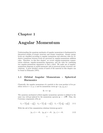
CHAPTER 1. ANGULAR MOMENTUM4zθryxφFigure 1.1: Transformation from rectangular to spherical coordinates.†, it follows thatSince J J J λ, mi η λ, m 1i,J λ, m 1i η λ, mi.Evaluating the expectation of J 2 J J Jz2 Jz in the state λ, mi, one finds η 2 j(j 1) m(m 1).Choosing the phase of η to be real and positive, leads to the relationsp(j m 1)(j m) λ, m 1i,J λ, mi p(j m 1)(j m) λ, m 1i.J λ, mi 1.1.2(1.18)(1.19)Spherical Coordinates - Spherical HarmonicsLet us apply the general results derived in Section 1.1.1 to the orbital angularmomentum operator L. For this purpose, it is most convenient to transformEqs.(1.1) to spherical coordinates (Fig. 1.1):x r sin θ cos φ,y r sin θ sin φ,pr x2 y 2 z 2 , θ arccos z/r,z r cos θ,φ arctan y/x.In spherical coordinates, the components of L areµ¶ cos φ cot θ,Lx ih̄ sin φ θ φµ¶ sin φ cot θ,Ly ih̄ cos φ θ φ Lz ih̄ , φ(1.20)(1.21)(1.22)

1.1. ORBITAL ANGULAR MOMENTUM - SPHERICAL HARMONICSand the square of the angular momentum isµ¶ 1 21 sin θ .L2 h̄2sin θ θ θ sin2 θ φ25(1.23)Combining the equations for Lx and Ly , we obtain the following expressions forthe orbital angular momentum raising and lowering operators:¶µ i cot θ.(1.24)L h̄e iφ θ φThe simultaneous eigenfunctions of L2 and Lz are called spherical harmonics.They are designated by Ylm (θ, φ). We decompose Ylm (θ, φ) into a product of afunction of θ and a function of φ:Ylm (θ, φ) Θl,m (θ)Φm (φ) .The eigenvalue equation Lz Yl,m (θ, φ) h̄mYl,m (θ, φ) leads to the equation idΦm (φ) mΦm (φ) ,dφ(1.25)for Φm (φ). The single valued solution to this equation, normalized so thatZ 2π Φm (φ) 2 dφ 1 ,(1.26)0is1Φm (φ) eimφ ,2π(1.27)where m is an integer. The eigenvalue equation L2 Yl,m (θ, φ) h̄2 l(l 1)Yl,m (θ, φ) leads to the differential equation¶µdm21 dsin θ (1.28) l(l 1)Θl,m (θ) 0 ,sin θ dθdθ sin2 θfor the function Θl,m (θ). The orbital angular momentum quantum number lmust be an integer since m is an integer.One can generate solutions to Eq.(1.28) by recurrence, starting with thesolution for m l and stepping forward in m using the raising operator L ,or starting with the solution for m l and stepping backward using the loweringoperator L . The function Θl, l (θ) satisfies the differential equation¶µd l cot θ Θl, l (θ) 0 ,L Θl, l (θ)Φ l (φ) h̄Φ l 1 (φ) dθwhich can be easily solved to give Θl, l (θ) c sinl θ, where c is an arbitraryconstant. Normalizing this solution so thatZ π Θl, l (θ) 2 sin θdθ 1,(1.29)0

CHAPTER 1. ANGULAR MOMENTUM6one obtains1Θl, l (θ) l2 l!r(2l 1)!sinl θ .2l mto Yl, l (θ, φ), leads to the resultApplying L s( 1)l m (2l 1)(l m)!dl mmsinθsin2l θ .Θl,m (θ) 2l l!2(l m)!d cos θl mFor m 0, this equation reduces tor( 1)l 2l 1 dlsin2l θ .Θl,0 (θ) l2 l!2 d cos θl(1.30)(1.31)(1.32)This equation may be conveniently written in terms of Legendre polynomialsPl (cos θ) asr2l 1Pl (cos θ) .(1.33)Θl,0 (θ) 2Here the Legendre polynomial Pl (x) is defined by Rodrigues’ formulaPl (x) 1 dl 2(x 1)l .2l l! dxlFor m l, Eq.(1.31) gives( 1)lΘl,l (θ) l2 l!r(2l 1)!sinl θ .2(1.34)(1.35)Starting with this equation and stepping backward l m times leads to analternate expression for Θl,m (θ):s( 1)l (2l 1)(l m)!dl msin m θsin2l θ .(1.36)Θl,m (θ) l2 l!2(l m)!d cos θl mComparing Eq.(1.36) with Eq.(1.31), one findsΘl, m (θ) ( 1)m Θl,m (θ) .(1.37)We can restrict our attention to Θl,m (θ) with m 0 and use (1.37) to obtainΘl,m (θ) for m 0. For positive values of m, Eq.(1.31) can be writtens(2l 1)(l m)! mPl (cos θ) ,(1.38)Θl,m (θ) ( 1)m2(l m)!where Plm (x) is an associated Legendre functions of the first kind, given inAbramowitz and Stegun (1964, chap. 8), with a different sign convention, definedbydm(1.39)Plm (x) (1 x2 )m/2 m Pl (x) .dx

1.2. SPIN ANGULAR MOMENTUM7The general orthonormality relations hl, m l0 , m0 i δll0 δmm0 for angular momentum eigenstates takes the specific formZ π Z 2π sin θdθdφ Yl,m(θ, φ)Yl0 ,m0 (θ, φ) δll0 δmm0 ,(1.40)00for spherical harmonics. Comparing Eq.(1.31) and Eq.(1.36) leads to the relation (θ, φ) .Yl, m (θ, φ) ( 1)m Yl,m(1.41)The first few spherical harmonics are:qY00 qY10 qY20 14π34π516πqcos θ(3 cos2 θ 1)15Y2, 2 32πsin2 θ e 2iφq7Y30 16πcos θ (5 cos2 θ 3)q105Y3, 2 32πcos θ sin2 θ e 2iφ1.21.2.1q3Y1, 1 8πsin θ e iφq15Y2, 1 8πsin θ cos θ e iφq21Y3, 1 64πsin θ (5 cos2 θ 1) e iφq35Y3, 3 64πsin3 θ e 3iφSpin Angular MomentumSpin 1/2 and SpinorsThe internal angular momentum of a particle in quantum mechanics is calledspin angular momentum and designated by S. Cartesian components of S satisfyangular momentum commutation rules (1.4). The eigenvalue of S 2 is h̄2 s(s 1)and the 2s 1 eigenvalues of Sz are h̄m with m s, s 1, · · · , s. Let usconsider the case s 1/2 which describes the spin of the electron. We designatethe eigenstates of S 2 and Sz by two-component vectors χµ , µ 1/2:µ ¶µ ¶10, χ 1/2 .(1.42)χ1/2 01These two-component spin eigenfunctions are called spinors. The spinors χµsatisfy the orthonormality relationsχ†µ χν δµν .The eigenvalue equations for S 2 and Sz areS 2 χµ 34 h̄2 χµ ,Sz χµ µh̄χµ .(1.43)

CHAPTER 1. ANGULAR MOMENTUM8We represent the operators S 2 and Sz as 2 2 matrices acting in the spacespanned by χµ :µ¶µ¶1 01 0.S 2 34 h̄2,Sz 12 h̄0 10 1One can use Eqs.(1.18,1.19) to work out the elements of the matrices representing the spin raising and lowering operators S :µ¶µ¶0 10 0,S h̄.S h̄0 01 0These matrices can be combined to give matrices representing Sx (S S )/2and Sy (S S )/2i. The matrices representing the components of S arecommonly written in terms of the Pauli matrices σ (σx , σy , σz ), which aregiven byµ¶µ¶µ¶0 10 i1 0, σy , σz ,(1.44)σx 1 0i 00 1through the relation1h̄σ .2The Pauli matrices are both hermitian and unitary. Therefore,S σx2 I, σy2 I, σz2 I,(1.45)(1.46)where I is the 2 2 identity matrix. Moreover, the Pauli matrices anticommute:σy σx σx σy , σz σy σy σz , σx σz σz σx .(1.47)The Pauli matrices also satisfy commutation relations that follow from the general angular momentum commutation relations (1.4):σx σy σy σx 2iσz ,σy σz σz σy 2iσx ,σz σx σx σz 2iσy .(1.48)The anticommutation relations (1.47) and commutation relations (1.48) can becombined to giveσx σy iσz ,σy σz iσx , σz σx iσy .(1.49)From the above equations for the Pauli matrices, one can showσ · a σ · b a · b iσ · [a b],(1.50)for any two vectors a and b.In subsequent studies we will require simultaneous eigenfunctions of L2 , Lz ,S 2 , and Sz . These eigenfunctions are given by Ylm (θ, φ) χµ .