Transcription
uncorrected preprintA Tutorial on Machine Learningand Data Science Tools with PythonMarcus D. Bloice(B) and Andreas HolzingerHolzinger Group HCI-KDD, Institute for Medical Informatics,Statistics and Documentation, Medical University of Graz, Graz, z.atAbstract. In this tutorial, we will provide an introduction to the mainPython software tools used for applying machine learning techniques tomedical data. The focus will be on open-source software that is freelyavailable and is cross platform. To aid the learning experience, a companion GitHub repository is available so that you can follow the examplescontained in this paper interactively using Jupyter notebooks. The notebooks will be more exhaustive than what is contained in this chapter,and will focus on medical datasets and healthcare problems. Briefly, thistutorial will first introduce Python as a language, and then describe someof the lower level, general matrix and data structure packages that arepopular in the machine learning and data science communities, such asNumPy and Pandas. From there, we will move to dedicated machinelearning software, such as SciKit-Learn. Finally we will introduce theKeras deep learning and neural networks library. The emphasis of thispaper is readability, with as little jargon used as possible. No previousexperience with machine learning is assumed. We will use openly available medical datasets throughout.Keywords: Machine learningTools · Languages · Python1·Deep learning·Neural networks·IntroductionThe target audience for this tutorial paper are those who wish to quickly getstarted in the area of data science and machine learning. We will provide anoverview of the current and most popular libraries with a focus on Python,however we will mention alternatives in other languages where appropriate. Alltools presented here are free and open source, and many are licensed under veryflexible terms (including, for example, commercial use). Each library will beintroduced, code will be shown, and typical use cases will be described. Medicaldatasets will be used to demonstrate several of the algorithms.Machine learning itself is a fast growing technical field [1] and is highly relevant topic in both academia and in the industry. It is therefore a relevant skill tohave in both academia and in the private sector. It is a field at the intersectionof informatics and statistics, tightly connected with data science and knowledgec Springer International Publishing AG 2016 A. Holzinger (Ed.): ML for Health Informatics, LNAI 9605, pp. 435–480, 2016.DOI: 10.1007/978-3-319-50478-0 22
436M.D. Bloice and A. Holzingerdiscovery [2,3]. The prerequisites for this tutorial are therefore a basic understanding of statistics, as well as some experience in any C-style language. Someknowledge of Python is useful but not a must.An accompanying GitHub repository is provided to aid the tutorial:https://github.com/mdbloice/MLDSIt contains a number of notebooks, one for each main section. The notebookswill be referred to where relevant.2Glossary and Key TermsThis section provides a quick reference for several algorithms that are not explicity mentioned in this chapter, but may be of interest to the reader. This shouldprovide the reader with some keywords or useful points of reference for othersimilar libraries to those discussed in this chapter.BIDMach GPU accelerated machine learning library for algorithms that arenot necessarily neural network based.Caret provides a standardised API for many of the most useful machine learning packages for R. See http://topepo.github.io/caret/index.html. For readers who are more comfortable with R, Caret provides a good substitute forPython’s SciKit-Learn.Mathematica is a commercial symbolic mathematical computation system,developed since 1988 by Wolfram, Inc. It provides powerful machine learningtechniques “out of the box” such as image classification [4].MATLAB is short for MATrix LABoratory, which is a commercial numerical computing environment, and is a proprietary programming language byMathWorks. It is very popular at universities where it is often licensed. It wasoriginally built on the idea that most computing applications in some wayrely on storage and manipulations of one fundamental object—the matrix,and this is still a popular approach [5].R is used extensively by the statistics community. The software package Caretprovides a standardised API for many of R’s machine learning libraries.WEKA is short for the Waikato Environment for Knowledge Analysis [6] andhas been a very popular open source tool since its inception in 1993. In 2005Weka received the SIGKDD Data Mining and Knowledge Discovery ServiceAward: it is easy to learn and simple to use, and provides a GUI to manymachine learning algorithms [7].Vowpal Wabbit Microsoft’s machine learning library. Mature and activelydeveloped, with an emphasis on performance.3Requirements and InstallationThe most convenient way of installing the Python requirements for this tutorialis by using the Anaconda scientific Python distribution. Anaconda is a collection
Tutorial on Machine Learning and Data Science437of the most commonly used Python packages preconfigured and ready to use.Approximately 150 scientific packages are included in the Anaconda installation.To install Anaconda, visithttps://www.continuum.io/downloadsand install the version of Anaconda for your operating system.All Python software described here is available for Windows, Linux, andMacintosh. All code samples presented in this tutorial were tested under UbuntuLinux 14.04 using Python 2.7. Some code examples may not work on Windowswithout slight modification (e.g. file paths in Windows use \ and not / as inUNIX type systems).The main software used in a typical Python machine learning pipeline canconsist of almost any combination of the following tools:1.2.3.4.5.NumPy, for matrix and vector manipulationPandas for time series and R-like DataFrame data structuresThe 2D plotting library matplotlibSciKit-Learn as a source for many machine learning algorithms and utilitiesKeras for neural networks and deep learningEach will be covered in this book chapter.3.1Managing PackagesAnaconda comes with its own built in package manager, known as Conda. Usingthe conda command from the terminal, you can download, update, and deletePython packages. Conda takes care of all dependencies and ensures that packagesare preconfigured to work with all other packages you may have installed.First, ensure you have installed Anaconda, as per the instructions underhttps://www.continuum.io/downloads.Keeping your Python distribution up to date and well maintained is essentialin this fast moving field. However, Anaconda makes it particularly easy to manage and keep your scientific stack up to date. Once Anaconda is installed youcan manage your Python distribution, and all the scientific packages installedby Anaconda using the conda application from the command line. To list allpackages currently installed, use conda list. This will output all packages andtheir version numbers. Updating all Anaconda packages in your system is performed using the conda update -all command. Conda itself can be updatedusing the conda update conda command, while Python can be updated usingthe conda update python command. To search for packages, use the searchparameter, e.g. conda search stats where stats is the name or partial nameof the package you are searching for.44.1Interactive Development EnvironmentsIPythonIPython is a REPL that is commonly used for Python development. It is includedin the Anaconda distribution. To start IPython, run:
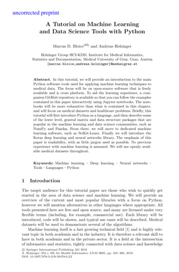
4381M.D. Bloice and A. Holzinger ipythonListing 1. Starting IPythonSome informational data will be displayed, similar to what is seen in Fig. 1,and you will then be presented with a command prompt.Fig. 1. The IPython Shell.IPython is what is known as a REPL: a Read Evaluate Print Loop. Theinterpreter allows you to type in commands which are evaluated as soon as youpress the Enter key. Any returned output is immediately shown in the console.For example, we may type the following:123456In [1]:Out [1]:In [2]:In [3]:Out [3]:In [4]:1 12import mathmath . radians (90)1.5707963267948966Listing 2. Examining the Read Evaluate Print Loop (REPL)After pressing return (Line 1 in Listing 2), Python immediately interprets theline and responds with the returned result (Line 2 in Listing 2). The interpreterthen awaits the next command, hence Read Evaluate Print Loop.Using IPython to experiment with code allows you to test ideas withoutneeding to create a file (e.g. fibonacci.py) and running this file from the command line (by typing python fibonacci.py at the command prompt). Usingthe IPython REPL, this entire process can be made much easier. Of course,creating permanent files is essential for larger projects.
Tutorial on Machine Learning and Data Science439A useful feature of IPython are the so-called magic functions. These commands are not interpreted as Python code by the REPL, instead they are specialcommands that IPython understands. For example, to run a Python script youcan use the %run magic function:12 % run fibonacci . py 30Fibonacci number 30 is 832040.Listing 3. Using the %run magic function to execute a file.In the code above, we have executed the Python code contained in the filefibonacci.py and passed the value 30 as an argument to the file.The file is executed as a Python script, and its output is displayed in theshell. Other magic functions include %timeit for timing code execution:123456 def fibonacci ( n ) :.if n 0: return 0.if n 1: return 1.return fibonacci (n -1) fibonacci (n -2) % timeit fibonacci (25)10 loops , best of 3: 30.9 ms per loopListing 4. The %timeit magic function can be used to check execution times offunctions or any other piece of code.As can be seen, executing the fibonacci(25) function takes on average30.9 ms. The %timeit magic function is clever in how many loops it performs tocreate an average result, this can be as few as 1 loop or as many as 10 millionloops.Other useful magic functions include %ls for listing files in the current working directory, %cd for printing or changing the current directory, and %cpastefor pasting in longer pieces of code that span multiple lines. A full list of magicfunctions can be displayed using, unsurprisingly, a magic function: type %magicto view all magic functions along with documentation for each one. A summaryof useful magic functions is shown in Table 1.Last, you can use the ? operator to display in-line help at any time. Forexample, typing123 abs ?Docstring :abs ( number ) - number456Return the absolute value of the argument .Type :builtin function or methodListing 5. Accessing help within the IPython console.For larger projects, or for projects that you may want to share, IPythonmay not be ideal. In Sect. 4.2 we discuss the web-based notebook IDE known asJupyter, which is more suited to larger projects or projects you might want toshare.
440M.D. Bloice and A. HolzingerTable 1. A non-comprehensive list of IPython magic functions.Magic Command Description%lsmagicLists all the magic functions%magicShows descriptive magic function documentation%lsLists files in the current directory%cdShows or changes the current directory%whoShows variables in scope%whosShows variables in scope along with type information%cpastePastes code that spans several lines%resetResets the session, removing all imports and deleting all variables%debugStarts a debugger post mortem4.2JupyterJupyter, previously known as IPython Notebook, is a web-based, interactive development environment. Originally developed for Python, it has sinceexpanded to support over 40 other programming languages including Juliaand R.Jupyter allows for notebooks to be written that contain text, live code, images,and equations. These notebooks can be shared, and can even be hosted onGitHub for free.For each section of this tutorial, you can download a Juypter notebook thatallows you to edit and experiment with the code and examples for each topic.Jupyter is part of the Anaconda distribution, it can be started from the commandline using using the jupyter command:1 jupyter notebookListing 6. Starting JupyterUpon typing this command the Jupyter server will start, and you will brieflysee some information messages, including, for example, the URL and port atwhich the server is running (by default http://localhost:8888/). Once theserver has started, it will then open your default browser and point it to thisaddress. This browser window will display the contents of the directory whereyou ran the command.To create a notebook and begin writing, click the New button and selectPython. A new notebook will appear in a new tab in the browser. A Jupyternotebook allows you to run code blocks and immediately see the output of theseblocks of code, much like the IPython REPL discussed in Sect. 4.1.Jupyter has a number of short-cuts to make navigating the notebook andentering code or text quickly and easily. For a list of short-cuts, use the menuHelp Keyboard Shortcuts.
Tutorial on Machine Learning and Data Science4.3441SpyderFor larger projects, often a fully fledged IDE is more useful than Juypter’snotebook-based IDE. For such purposes, the Spyder IDE is often used.Spyder stands for Scientific PYthon Development EnviRonment, and is includedin the Anaconda distribution. It can be started by typing spyder in the command line.5Requirements and ConventionsThis tutorial makes use of a number of packages which are used extensively inthe Python machine learning community. In this chapter, the NumPy, Pandas,and Matplotlib are used throughout. Therefore, for the Python code samplesshown in each section, we will presume that the following packages are availableand have been loaded before each script is run:123 import numpy as np import pandas as pd import matplotlib . pyplot as pltListing 7. Standard libraries used throughout this chapter. Throughout this chapterwe will assume these libraries have been imported before each script.Any further packages will be explicitly loaded in each code sample. However,in general you should probably follow each section’s Jupyter notebook as youare reading.In Python code blocks, lines that begin with represent Python codethat should be entered into a Python interpreter (See Listing 7 for an example).Output from any Python code is shown without any preceding characters.Commands which need to be entered into the terminal (e.g. bash or theMS-DOS command prompt) begin with , such as:12345 l s lAht o t a l 299K rw rw r 1 b l o i c e admin rw rw r 1 b l o i c e admin.73K Sep 1 1 4 : 1 1 C l u s t e r i n g . ipynb57K Aug 25 1 6 : 0 4 Pandas . ipynbListing 8. Commands for the terminal are preceded by a sign.Output from the console is shown without a preceding sign. Some of thecommands in this chapter may only work under Linux (such as the example usageof the ls command in the code listing above, the equivalent in Windows is thedir command). Most commands will, however, work under Linux, Macintosh,and Windows—if this is not the case, we will explicitly say so.5.1DataFor the Introduction to Python, NumPy, and Pandas sections we will work witheither generated data or with a toy dataset. Later in the chapter, we will move
442M.D. Bloice and A. Holzingeron to medical examples, including a breast cancer dataset, a diabetes dataset,and a high-dimensional gene expression dataset. All medical datasets used inthis chapter are freely available and we will describe how to get the data ineach relevant section. In earlier sections, generated data will suffice in order todemonstrate example usage, while later we will see that analysing more involvedmedical data using the same open-source tools is equally possible.6Introduction to PythonPython is a general purpose programming language that is used for anythingfrom web-development to deep learning. According to several metrics, it is rankedas one of the top three most popular languages. It is now the most frequentlytaught introductory language at top U.S. universities according to a recent ACMblog article [8]. Due to its popularity, Python has a thriving open source community, and there are over 80,000 free software packages available for the languageon the official Python Package Index (PyPI).In this section we will give a very short crash course on using Python. Thesecode samples will work best with a Python REPL interpreter, such as IPythonor Jupyter (Sects. 4.1 and 4.2 respectively). In the code below we introduce thesome simple arithmetic syntax:12345678 80 1 1.5 2562 6 (8 * 9)3 / 23.0 / 24 ** 4 # To the power ofListing 9. Simple arithmetic with Python in the IPython shell.Python is a dynamically typed language, so you do not define the type ofvariable you are creating, it is inferred:1234567891011 n 5 f 5.5 s " 5 " type ( s )str type ( f )float " 5 " * 5" 55555 " int ( " 5 " ) * 525Listing 10. Demonstrating types in Python.
Tutorial on Machine Learning and Data Science443You can check types using the built-in type function. Python does awaywith much of the verbosity of languages such as Java, you do not even need tosurround code blocks with brackets or braces: if " 5 " 5:.print ( " Will not get here " ) elif int ( " 5 " ) 5:.print ( " Got here " )Got here12345Listing 11. Statement blocks in Python are indicated using indentation.As you can see, we use indentation to define our statement blocks. This is thenumber one source of confusion among those new to Python, so it is important youare aware of it. Also, whereas assignment uses , we check equality using (andinversely ! ). Control of flow is handled by if, elif, while, for, and so on.While there are several basic data structures, here we will concentrate on listsand dictionaries (we will cover much more on data structures in Sect. 7.1). Othertypes of data structures are, for example, tuples, which are immutable—theircontents cannot be changed after they are created—and sets, where repetition isnot permitted. We will not cover tuples or sets in this tutorial chapter, however.Below we first define a list and then perform a number of operations on thislist:123456789101112131415161718 powers [1 , 2 , 4 , 8 , 16 , 32] powers[1 , 2 , 4 , 8 , 16 , 32] powers [0]1 powers . append (64) powers[1 , 2 , 4 , 8 , 16 , 32 , 64] powers . insert (0 , 0) powers[0 , 1 , 2 , 4 , 8 , 16 , 32 , 64] del powers [0] powers[1 , 2 , 4 , 8 , 16 , 32 , 64] 1 in powersTrue 100 not in powersTrueListing 12. Operations on lists.Lists are defined using square [] brackets. You can index a list using itsnumerical, zero-based index, as seen on Line 4. Adding values is performed usingthe append and insert functions. The insert function allows you to define inwhich position you would like the item to be inserted—on Line 9 of Listing 12we insert the number 0 at position 0. On Lines 15 and 17, you can see how wecan use the in keyword to check for membership.
444M.D. Bloice and A. HolzingerYou just saw that lists are indexed using zero-based numbering, we will nowintroduce dictionaries which are key-based. Data in dictionaries are stored usingkey-value pairs, and are indexed by the keys that you define:12345678910 numbers { " bingo " : 3458080 , " tuppy " : 3459090} numbers{ " bingo " : 3458080 , " tuppy " : 3459090} numbers [ " bingo " ]3458080 numbers [ " monty " ] 3456060 numbers{ " bingo " : 3458080 , " monty " : 3456060 , " tuppy " : 3459090} " tuppy " in numbersTrueListing 13. Dictionaries in Python.We use curly {} braces to define dictionaries, and we must define both theirvalues and their indices (Line 1). We can access elements of a dictionary usingtheir keys, as in Line 4. On Line 6 we insert a new key-value pair. Notice thatdictionaries are not ordered. On Line 9 we can also use the in keyword to checkfor membership.To traverse through a dictionary, we use a for statement in conjunction witha function depending on what data we wish to access from the dictionary:12345 for name , number in numbers . iteritems () :.print ( " Name : " name " , number : " str ( number ) )Name : bingo , number : 3458080Name : monty , number : 3456060Name : tuppy , number : 345909067891011 for key in numbers . keys () :.print ( key )bingomontytuppy121314151617 for val in numbers . values () :.print ( val )345808034560603459090Listing 14. Iterating through dictionaries.First, the code above traverses through each key-value pair usingiteritems() (Line 1). When doing so, you can specify a variable name foreach key and value (in that order). In other words, on Line 1, we have statedthat we wish to store each key in the variable name and each value in the variable number as we go through the for loop. You can also access only the keysor values using the keys and values functions respectively (Lines 7 and 13).
Tutorial on Machine Learning and Data Science445As mentioned previously, many packages are available for Python. These needto be loaded into the current environment before they are used. For example,the code below uses the os module, which we must first import before using:12345678910111213 import os os . listdir ( " ./ " )[ " BookChapter . ipynb " ," NumPy . ipynb " ," Pandas . ipynb " ," fibonacci . py " ," LinearRegression . ipynb " ," Clustering . ipynb " ] from os import listdir # Alternatively listdir ( " ./ " )[ " BookChapter . ipynb " ," NumPy . ipynb " ,.Listing 15. Importing packages using the import keyword.Two ways of importing are shown here. On Line 1 we are importing the entireos name space. This means we need to call functions using the os.listdir()syntax. If you know that you only need one function or submodule you canimport it individually using the method shown on Line 9. This is often thepreferred method of importing in Python.Lastly, we will briefly see how functions are defined using the def keyword:1234 def addNumbers (x , y ) :.return x y addNumbers (4 , 2)6Listing 16. Functions are defined using the def keyword.Notice that you do not need to define the return type, or the arguments’types. Classes are equally easy to define, and this is done using the class keyword. We will not cover classes in this tutorial. Classes are generally arrangedinto modules, and further into packages. Now that we have covered some of thebasics of Python, we will move on to more advanced data structures such as2-dimensional arrays and data frames.77.1Handling DataData Structures and NotationIn machine learning, more often than not the data that you analyse will be storedin matrices and vectors. Generally speaking, your data that you wish to analysewill be stored in the form of a matrix, often denoted using a bold upper casesymbol, generally X, and your label data will be stored in a vector, denoted witha lower case bold symbol, often y.
446M.D. Bloice and A. HolzingerA data matrix X with n samples and m features x1,1 x1,2 x1,3 . . . x2,1 x2,2 x2,3 . . . X Rn m x3,1 x3,2 x3,3 . . . . . . .is denoted as follows: x1,mx2,m x3,m . . xn,1 xn,2 xn,3 . . . xn,mEach column, m, of this matrix contains the features of your data and eachrow, n, is a sample of your data. A single sample of your data is denoted by itssubscript, e.g. xi [xi,1 xi,2 xi,3 · · · xi,m ]In supervised learning, your labels or targets are stored in a vector: y1 y2 y Rn 1 y3 . . ynNote that number of elements in the vector y is equal to the number ofsamples n in your data matrix X, hence y Rn 1 .For a concrete example, let us look at the famous Iris dataset. The Iris flowerdataset is a small toy dataset consisting of n 150 samples or observations ofthree species of Iris flower (Iris setosa, Iris virginica, and Iris versicolor). Eachsample, or row, has m 4 features, which are measurements relating to thatsample, such as the petal length and petal width. Therefore, the features of theIris dataset correspond to the columns in Table 2, namely sepal length, sepalwidth, petal length, and petal width. Each observation or sample corresponds toone row in the table. Table 2 shows a few rows of the Iris dataset so that you canbecome acquainted with how it is structured. As we will be using this datasetin several sections of this chapter, take a few moments to examine it.Table 2. The Iris flower dataset.Sepal length Sepal width Petal length Petal width .2.1.3.0.2.setosa.150 5.93.05.11.8virginicaIn a machine learning task, you would store this table in a matrix X, whereX R150 4 . In Python X would therefore be stored in a 2-dimensional array
Tutorial on Machine Learning and Data Science447with 150 rows and 4 columns (generally we will store such data in a variablenamed X). The 1st row in Table 2 corresponds to 1st row of X, namely x1 [5.1 3.5 1.4 0.2]. See Listing 17 for how to represent a vector as an array anda matrix as a two-dimensional array in Python. While the data is stored in amatrix X, the Class column in Table 2, which represents the species of plant, isstored separately in a target vector y. This vector contains what are known as thetargets or labels of your dataset. In the Iris dataset, y [y1 y2 · · · y150 ], yi {setosa, versicolor, virginica}. The labels can either be nominal, as is the casein the Iris dataset, or continuous. In a supervised machine learning problem,the principle aim is to predict the label for a given sample. If the targetsare nominal, this is a classification problem. If the targets are continuous thisis a regression problem. In an unsupervised machine learning task you do nothave the target vector y, and you only have access to the dataset X. In such ascenario, the aim is to find patterns in the dataset X and cluster observationstogether, for example.We will see examples of both classification algorithms and regression algorithms in this chapter as well as supervised and unsupervised problems.12345 v1 [5.1 , 3.5 , 1.4 , 0.2] v2 [.[5.1 , 3.5 , 1.4 , 0.2] ,.[4.9 , 3.0 , 1.3 , 0.2].]Listing 17. Creating 1-dimensional (v1) and 2-dimensional data structures (v2) inPython (Note that in Python these are called lists).In situations where your data is split into subsets, such as a training set anda test set, you will see notation such as Xtrain and Xtest . Datasets are often splitinto a training set and a test set, where the training set is used to learn a model,and the test set is used to check how well the model fits to unseen data.In a machine learning task, you will almost always be using a libraryknown as NumPy to handle vectors and matrices. NumPy provides very useful matrix manipulation and data structure functionality and is optimised forspeed. NumPy is the de facto standard for data input, storage, and output inthe Python machine learning and data science community1 . Another importantlibrary which is frequently used is the Pandas library for time series and tabulardata structures. These packages compliment each other, and are often used sideby side in a typical data science stack. We will learn the basics of NumPy andPandas in this chapter, starting with NumPy in Sect. 7.2.1To speed up certain numerical operations, the numexpr and bottleneck optimisedlibraries for Python can be installed. These are included in the Anaconda distribution, readers who are not using Anaconda are recommended to install them both.
4487.2M.D. Bloice and A. HolzingerNumPyNumPy is a general data structures, linear algebra, and matrix manipulationlibrary for Python. Its syntax, and how it handles data structures and matricesis comparable to that of MATLAB2 .To use NumPy, first import it (the convention is to import it as np, to avoidhaving to type out numpy each time): import numpy as np1Listing 18. Importing NumPy. It is convention to import NumPy as np.Rather than repeat this line for each code listing, we will assume you haveimported NumPy, as per the instructions in Sect. 3. Any further imports thatmay be required for a code sample will be explicitly mentioned.Listing 19 describes some basic usage of NumPy by first creating a NumPyarray and then retrieving some of the elements of this array using a techniquecalled array slicing:1234567891011 [0 , 1 [0 , [0 , [3 ,vector np . arange (10) # Make an array from 0 - 9vector1 , 2 , 3 , 4 , 5 , 6 , 7 , 8 , 9]vector [1]vector [0:3]1 , 2]vector [0: -3] # Element 0 to the 3 rd last element1 , 2 , 3 , 4 , 5 , 6]vector [3:7] # From index 3 but not including 74 , 5 , 6]Listing 19. Array slicing in NumPy.In Listing 19, Line 1 we have created a vector (actually a NumPy array)with 10 elements from 0–9. On Line 2 we simply print the contents of thevector, the contents of which are shown on Line 3. Arrays in Python are 0indexed, that means to retrieve the first element you must use the number 0. OnLine 4 we retrieve the 2nd element which is 1, using the square bracket indexing syntax: array[i], where i is the index of the value you wish to retrievefrom array. To retrieve subsets of arrays we use a method known as array slicing, a powerful technique that you will use constantly, so it is worthwhile tostudy its usage carefully! For example, on Line 9 we are retrieving all elementsbeginning with element 0 to the 3rd last element. Slicing 1D arrays takes theform array[ startpos : endpos ], where the start position startpos andend position endpos are separated with a: character. Line 11 shows anotherexample of array slicing. Array slicing includes the element indexed by the startpos up to but not including the element indexed by endpos .2Users of MATLAB may want to view this excellent guide to NumPy for MATLABusers: ml.
Tutor
experience with machine learning is assumed. We will use openly avail-able medical datasets throughout. Keywords: Machine learning · Deep learning · Neural networks · Tools · Languages · Python 1 Introduction The target audience for this tutorial paper are those who wish to quickly get started in the area of data science and machine learning.