Transcription
2.15COASTAL WAVE PREDICTION FOR CAPE CANAVERAL, FLORIDAAndrew T. Cox* and Vincent J. CardoneOceanweather Inc., Cos Cob, CTDon T. ResioWaterways Experiment Station, Vicksburg, MS1. INTRODUCTION2. WAVE MODELSDuring May 1999, the Rapidly InstalledBreakwater System (RIBS) was tested by the U.S.Army Waterways Experiment Station (WES) inocean trials held just offshore of Cape Canaveral,Florida. RIBS is a movable breakwater designedto increase the range of wave heights in which theU.S. armed forces can offload ships duringLogistics Over The Shore (LOTS) operations. TheRIBS experiment used a prototype RIB to test thesurvivability, deployment options, and mooring ofthe breakwater. Data from this trial will be used todevelop a final design for RIBS.Three nested wave models were used tomake the RIBS forecast. North Atlantic swellswere provided from Oceanweather's global wavemodel, which runs on a 1.25 by 2.5 degreelatitude/longitude grid. Wind inputs for the globalmodel were derived separately from the RIBSwind fields (as described in section 3). However,the wind generation techniques were similar. Aregional model (Figure 1) on a 28 km grid wasused to better resolve the islands of the Bahamaswhich are not resolved on the global grid. Theglobal and 28 km regional wave models used theso-called ODGP2 fully discrete spectral wavemodel (OWI-1G). The spectrum is resolved ateach grid point in 24 directional bins and 23frequency bins. Deep water physics is assumed inboth the propagation algorithm and source terms.More details on the OWI-1G model can be foundin Khandekar et al. (1994).As part of the RIBS experiment, detailedpredictions of sea-state were required for the safedeployment and operation of the movablebreakwater. This paper describes the coastalwave prediction system developed to make theseforecasts. The prediction system consisted ofthree nested wave models, the finest includingshallow water effects on a 2.775 km grid. Windsdriving the RIBS wave models are derived fromthe Wind WorkStation (WWS) which blends modeldata, in situ measurements and forecaster's inputsusing the Interactive Objective Kinematic Analysis(IOKA) algorithm. Model inputs evaluated by theforecasterincludeNationalCenterforEnvironmental Prediction (NCEP) Aviation andETA 10-meter wind fields. In-situ windobservations include NOAA buoys, ship reports,CMAN stations, NWS reporting stations, ERS-2scatterometer winds, and Kennedy SpaceflightCenter (KSC) tower winds.Validation wasperformed against both the Cape CanaveralNOAA buoy and a buoy deployed at the RIBSlocation.*Corresponding author address: Andrew T. Cox,Oceanweather Inc., Cos Cob, CT 06807;e-mail:andrewc@oceanweather.comFigure 1. 28 km wave model grid.
and for each frequency and direction bin, anumerical shallow-water tracing program wasused instead of the simple great circle ray-pathcomputation used in the deep-water model.Effects of shoaling and refraction over an irregularbathymetry as resolved on the fine grid aretherefore resolved. The bathymetry was obtainedfrom manually digitized NOAA coastal surveymaps.Along the boundaries of the 28 km and 2.775km grids the time histories of full two-dimensionalwave spectra were interpolated in space from thelower resolution grid to the higher resolution grid.3. WIND INPUTSFigure 2. 2.775 km wave model grid with depth contours inmeters.A shallow water version of OWI-1G wasimplemented on a 2.775 km grid (Figure 2) toprovide wave forecasts at the RIBS location.OWI-1G was first extended to shallow water in themid-1980s and first tested against measured datain a shallow environment during the CanadianAtlantic Storms Project (CASP). The performanceof the model hindcasts was shown to exceed thatof several other operational and research shallowwater wave models which participated in thatexperiment (Eid and Cardone, 1987).The modifications of the ODGP deep-watersource term algorithm for shallow water include (1)transformation of the asymptotic limit to growth: (2)addition of an explicit bottom friction source termmodeled after the treatment of Grant and Madsen(1982) ; calculation of the exponential growth rateusing the shallow-water celerity; adoption of wavenumber scaling of the saturation range of thespectrum, with the equilibrium range coefficientexpressed as a function of the stage of wavedevelopment.The propagation scheme of the shallow watermodel is analagous to that used in the deep watermodel, which uses a precomputed table ofpropagation coefficients. In the construction of thetable of propagation coefficients at each grid pointWind fields for the RIBS 28 km and 2.775 kmwave models were derived using an interactiveWind Workstation (WWS, Cox et al., 1995). TheWWS allows an analyst to blend model winds,measured winds, and forecaster inputs using theapproach described by Cardone et al. (1995,1996).NCEP's Aviation and ETA 28 km 10-meterwind fields were used as the primary model input.In-situ marine wind measurements consisted ofNOAA buoys, CMAN stations, and ship reports.Winds were adjusted for height and stability to areference level of 10 meters using the methoddescribedbyCardoneetal.(1990).Scatterometer winds were obtained in real-timefrom the ERS-2 instrument, these winds werealready at a 10-meter reference height and did notrequire any further modification. Coastal NWSreporting stations, and wind tower data from theKennedy Spaceflight Center (KSC) were also usedfor defining the wind fields in the near-shoreregion. Figure 3 shows a typical analysis map, thecluster of land observations over Cape Canaveralis from the KSC wind tower data. Most of thetowers were located on the coast and hadexcellent marine exposure.In the analysis domain, model wind fields weremodified as indicated by the in situ observationsusing classical kinematic techniques.In theforecast domain, continuity from the analysis mapswas maintained and additional model data fromthe NGM, FNOC, and ECMWF models wasevaluated for possible inclusion.Maps weremodified every 6 hours from -24 to 48 hours, thenevery 12 hours out to 72. Wind fields were then
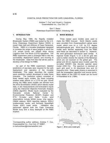
Figure 3. WWS display showing gridded AVN and ETA winds, contoured AVN pressures with in situ data from buoys, ships,CMAN Stations, and KSC tower winds.time interpolated for the 28 km and 2.775 km wavemodels.4. WAVE MODEL VERIFICATIONFigure 4 shows wave model output contouredthevery 10 cm for May-17 at 12 GMT. A strongpressure gradient driving high northeast winds justoffshore the Carolina's generated the swells whichpropagated down the coast into the RIBS domain.Wave model verification for the RIBS forecastconsisted of the NOAA Buoy 41009 and wavemeasurements made at the RIBS location. Buoy41009 is located 37 km East of Cape Canaveral in42 m of water. The RIBS buoy is located justoffshore of Cape Canaveral in 9 meters of water.Wave measurements were smoothed using a /1-hour time window. All comparisons were madeusing the high-resolution 2.775 km wave modeloutput.Figure 5 shows the time series comparison ofsignificant wave height forecasts and analysisagainst buoy 41009. There were three eventsduring the RIBS trial period with sea states aboveFigure 4. Significant wave height contours every 10 cm.
Significant Wave HeightSignificant Wave HeightSignificant Wave Height4MeasuredAnalysis 12Measured 24 36Measured 48 7232104321043210May 991 May8 Sat15 Sat22 Sat1 JunFigure 5. Comparison of model waves at buoy 41009.Significant Wave HeightSignificant Wave HeightSignificant Wave Height4MeasuredAnalysis 12Measured 24 36Measured 48 7232104321043210May 991 May8 Sat15 Sat22 SatFigure 6. Comparison of model waves at the RIBS buoy.1 Jun
thresholds which could potentially affect decisionsregarding the deployment, operation or retrieval ofthe RIBS: May 2, May 17, May 30. In general, thecomparisons show excellent agreement.ThendMay2 event was over-predicted in the 24 and 72 hour taus, but correctly modeled in theanalysis. The same time period at the RIBS buoy(Figure 6) also shows good agreement betweenthe measured and modeled waves. The modeltended to run slightly higher than themeasurements overall, but correctly predicted themain storm systems. Table 1 shows comparisonstatistics stratified by forecast horizon for both theNOAA buoy and RIBS buoy. Overall, the modelanalysis is slightly high at both locations (8 cm at41009 and 12 cm at the RIBS location) withscatter indices of .24 and .28, respectively.Table 1. Wave comparison statistics at buoys 41009 andRIBS. Bias is model-measured in meters, SI is scatterindex and CC is correlation coefficient.Buoy 41009RIBS BuoyTau# PtsBiasSICC# PtsBiasSICC02430.080.240.952070.120.280.89 12310.080.250.94250.080.260.81 24310.080.380.93260.120.280.82 36300.360.300.95250.130.320.69 48310.120.500.91260.110.260.85 72310.190.450.84260.190.490.445. CONCLUSIONSIn this paper, a coastal wave predictionsystem for Cape Canaveral, Florida wasdescribed. The system used a tri-nested spectralwave model and forecaster modified wind fields toproduce daily 72 hour wave forecasts for the RIBSexperiment. Verification against both the NOAAbuoy 41009 and RIBS buoy in the month of Mayshowed good agreement in both the analysis andforecast waves.The authors would like to thank the KennedythSpaceflight Meteorology Group and the 45Weather Squadron for making the KSC tower winddata available for this experiment.6. REFERENCESCardone, V.J., J.G. Greenwood and M.A. Cane,1990. On trends in historical marine wind data.J. of Climate, 3, 113-127.Cardone, V.J., H.C. Graber, R.E. Jensen, S.Hasselmann, M.J. Caruso, 1995. In search ofthe true surface wind field in SWADE IOP-1:ocean wave modelling perspective. TheGlobal Ocean Atmopshere System, 3, 107150.Cardone, V.J., R.E. Jensen, D.T. Resio, V.R.Swail and A.T. Cox, 1996. Evaluation ofContemporary Ocean Wave Models in RareExtreme Events: "Halloween Storm ofOctober, 1991; "Storm of the Century" ofMarch, 1993". J. Atmos. and Oceanic Tech.,Vol. 13, No. 1, p. 198-230.Cox, A.T., J.A. Greenwood, V.J. Cardone and V.R.Swail, 1995. An interactive objective kinematicanalysis system. Proceedings 4th InternationalWorkshop on Wave Hindcasting andForecasting, October 16-20, 1995, Banff,Alberta, p. 109-118.Eid, B. M., V. J. Cardone, J. A. Greenwood and J.Saunders. 1987. Real-time spectral waveforecasting model test during CASP. ESRFReport 065: Proceedings of the InternationalWorkshop on Wave Hindcasting andForecasting, September 23-26, 1996, Halifax,NS, 183-195.Grant, W. D. and O.S. Madsen, 1982: Movablebed roughness in unsteady oscillatory flow. J.of Geophys. Res. 87, C1, 469-481.Khandekar, M.L., R. Lalbeharry and V.J. Cardone,1994. The Performance of the CanadianSpectral Ocean Wave Model (CSOWM)During the Grand Banks ERS-1 SAR WaveSpectra Validation Experiment. AtmosphereOcean 31 (1), pp. 31-60.
Center (KSC) tower winds. Validation was performed against both the Cape Canaveral NOAA buoy and a buoy deployed at the RIBS location. *Corresponding author address: Andrew T. Cox, Oceanweather Inc., Cos Cob, CT 06807; e-mail:andrewc@oceanweather.com 2. WAVE MODELS Three nested wave models were used to make the RIBS forecast. North Atlantic swells