Transcription
HICSS-35: 35th Hawaii International Conference on System SciencesInteractive Visualization and Analysis for Gene Expression DataChun Tang, Li Zhang and Aidong ZhangDepartment of Computer Science and EngineeringThe State University of New York at BuffaloBuffalo, NY 14260chuntang, lizhang, azhang @cse.buffalo.eduAbstractNew technology such as DNA microarray can be used to produce the expression levels of thousandsof genes simultaneously. The raw microarray data are images which can be transformed into geneexpression matrices where usually the rows represent genes, the columns represent various samples, andthe number in each cell characterizes the expression level of the particular gene in a particular sample.Now the cDNA and genomic sequence projects are processing at such a rapid rate, more and more databecome available to researchers who are working in the field of bioinformatics. New methods are neededto efficiently and effectively analyze and visualize the gene data.A key step in the analysis of gene expression data is the detection of groups that manifest similarexpression patterns and filter out the genes that are inferred to represent noise from the matrix accordingto samples distribution. In this paper, we present a visualization method which maps the samples’ dimensional gene vectors into 2-dimensional points. This mapping is effective in keeping correlationcoefficient similarity which is the most suitable similarity measure for analyzing the gene expressiondata. Our analysis method first removes noise genes from the gene expression matrix by sorting genesaccording to correlation coefficient measure and then adjusts the weight for each remaining gene. Wehave integrated our gene analysis algorithm into a visualization tool based on this mapping method. Wecan use this tool to monitor the analysis procedure, to adjust parameters dynamically, and to evaluate theresult of each step. The experiments based on two groups of multiple sclerosis (MS) and treatment datademonstrate the effectiveness of this approach.1
1 IntroductionDNA microarray technology can be used to measure expression levels for thousands of genes in a singleexperiment, across different conditions and over time [3, 16, 14, 24, 23, 27, 36, 20, 21, 8, 30]. To usethe arrays, labeled cDNA is prepared from total messenger RNA (mRNA) of target cells or tissues, andis hybridized to the array. The amount of label bound is an approximate measure of the level of geneexpression. Thus gene microarrays can give a simultaneous, semi-quantitative readout on the levels ofexpressions of thousands of genes. Just 4-6 such high-density “gene chips” could allow rapid scanning ofthe entire human library for genes which are induced or repressed under particular conditions. By preparingcDNA from cells or tissues at intervals following some stimulus, and exposing each to replicate microarrays,it is possible to determine the identity of genes responding to that stimulus, the time course of induction,and the degree of change.Some methods have been developed using both standard cluster analysis and new innovative techniquesto extract, analyze and visualize gene expression data generated from DNA microarrays. Gene expressionmatrix can be studied in two dimensions [2]: comparing expression profiles of genes by comparing rowsin the expression matrix [22, 6, 26, 23, 25, 9, 33, 3] and comparing expression profiles of samples bycomparing columns in the matrix [?, 10, 32]. In addition, both methods can be combined (provided that thedata normalization [18, 38] allows it).A key step in the analysis of gene expression data is the detection of groups that manifest similar expression patterns and filter out the genes that are inferred to represent noise from the matrix according tosamples distribution. The corresponding algorithmic problem is to cluster multi-condition gene expressionpatterns. Data clustering [6] was used to identify patterns of gene expression in human mammary epithelial2
cells growing in culture and in primary human breast tumors. DeRisi et al. [17] used a DNA array containing a complete set of yeast genes to study the diauxic shift time course. They selected small groups of geneswith similar expression profiles and showed that these genes are functionally related and contain relevanttranscription factor binding sites upstream of their open reading frames (ORFs). In [3], a clustering algorithm was introduced for analysis of gene expression data in which an appropriate stochastic error modelon the input has been defined. Self-organizing maps [26, 19], a type of mathematical cluster analysis that issuited for recognizing and classifying features in complex, multidimensional data, was applied to organizethe genes into biologically relevant clusters that suggest novel hypotheses about hematopoietic differentiation. In [12], the authors presented a strategy for the analysis of large-scale quantitative gene-expressionmeasurement data from time-course experiments. The correlated patterns of gene expression from timeseries data suggests an order that conforms to a notion of shared pathways and control processes that canbe experimentally verified. Brown et al. [23] applied a method based on the theory of support vector machines (SVMs). The method is considered as a supervised computer learning method because it exploitsprior knowledge of gene function to identify unknown genes of similar function from expression data. Theyapplied this algorithm on six functional classes of yeast gene expression matrices from 79 samples [22]. Alter et al. [25] used singular value decomposition in transforming genome-wide expression data from genes arrays space to reduced diagonalized “eigengenes” “eigenarrays” space to extract significant genes bynormalizing and sorting the data. Hastie et al. [33] proposed a tree harvesting method for supervised learning from gene expression data. This technique starts with a hierarchical clustering of genes, then modelsthe outcome variable as a sum of the average expression profiles of chosen clusters and their products. Themethod can discover genes that have strong effects on their own, and genes that interact with other genes.On sample dimension, our task is to build a classifier which can predict the sample labels from the3
expression profile. Golub et al. [32] applied neighborhood analysis to construct class predictors for samples,especially for leukemias. They were looking for genes whose expression data are best correlated with twoknown classes of leukemias, acute myeloid leukemia and acute lymphoblastic leukemia. They constructeda weighted vote classifier based on 50 genes (out of 6817) using 38 samples and applied it to a collection of34 new samples. The classifier correctly predicted 29 of the 34 samples. In [10], the authors present a neuralnetwork model known as Simplified Fuzzy ARTMAP which can identify normal and diffuse large B-celllymphoma (DLBCL) patients using DNA microarrays data generated by a previous study. Many traditionalclustering algorithms such as the hierarchical [22, 15, 5] and K-means clustering algorithms [13, 28] have allbeen used for clustering expression profiles. Mathematical and statistical methods like Fourier and Bayesiananalysis also have been used to discover profiles of cell cycle-dependent genes [31, 37, 1]. Our group hasdeveloped a maximum entropy approach to classifying gene array data sets [29]. We used part of pre-knownclasses of samples as training set and applied the maximum entropy model to generate an optimal patternmodel which can be used to new samples.Sample clustering has been combined with gene clustering to identify which genes are the most important for sample clustering [34, 5]. Alon et al. [34] have applied a partitioning-based clustering algorithmto study 6500 genes of 40 tumor and 22 normal colon tissues for clustering both genes and samples. Getzet al. [11] present a method applied on colon cancer and leukemia data. By identifying relevant subsets ofthe data, they were able to discover partitions and correlations that were masked and hidden when the fulldataset was used in the analysis. This method is called two-way clustering.Multiple sclerosis (MS) is a chronic, relapsing, inflammatory disease. Interferon- ( ) has beenthe most important treatment for the MS disease for the last decade [35]. The DNA microarray technologymakes it possible to study the expression levels of thousands of genes simultaneously. The gene expression4
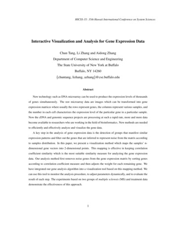
levels are measured by the intensity levels of the corresponding array spots. In this paper, we present avisualization method which maps the samples’ -dimension gene vectors into 2-dimensional points. Thismapping is effective in keeping correlation coefficient similarity which is the most suitable similarity measure for analyzing gene expression data. Our gene expression data analysis method first removes noise genesfrom the expression matrix by sorting genes according to correlation coefficient measure and then adjuststhe weight for each remaining gene. We have integrated our gene analysis algorithm into a visualization toolbased on this mapping method. We can use this tool to monitor the analysis procedure, to adjust parameters,and to evaluate the result of each step. The experiments on the healthy control, MS and IFN-treated samplesbased on the data collected from the DNA microarray experiments demonstrate the effectiveness of thisapproach.This paper is organized as follows. Section 2 introduces the visualization method. Section 3 describesthe details of our gene data analyzing approach with the help of our visualization tool. Section 4 presentsthe experimental results. And finally, the conclusion is provided in Section 5.2 Visualization Tool2.1 Mapping MethodA typical gene expression matrix has thousands of rows (each row represents a gene) and several (usuallyless than 100) columns which represent samples related to a certain kind of disease or other condition. Eachsample is marked with a label that points out which class it belongs to, such as control, patient and drugtreated. While we analyze these samples, we usually want to view the sample distribution during each step.How to visualize arbitrarily large dimensional data effectively and efficiently is still an open problem. Theparallel coordinate system allows the visualization of multidimensional data by a simple two dimensional5
Figure 1: Distribution of our gene expression data of 44 samples, where each samples has 4132 genes. (A) Visualization using the parallel coordinate system, where the horizontal axis represents gene dimension and each multidimensional line represent a sample. The sample distribution is not clear. (B) Visualization using our tool, where each pointrepresents a sample. The figure shows that after mapping original data into 2-dimensional space, sample distributionis clearly represented.representation. But as the dimensions go higher, the displaying is less effective. Figure 1 shows an exampleof different visualization methods.We use the idea of a linear mapping method that maps the multidimensional dataset to 2-dimensional ! "#"#" &%('space [7]. Let vector represent a data point in -dimensional space, and total numberof points in the space is ) , denoted as & "#"#"# & *. , We use the Formula (1) to map into a 2-dimensional point : , ./ 0.21 354'1. ' ' 6 (1)354is an adjustable weight for each coordinate, is vector length of the original space,is a ratio.6 78 :9! ; "#"#"# 'to centralize the points, and are unit vectors which divide the center circle of the displaywhere0%-.screen equally (Figure 2 (B)).6
Figure 2: Mapping from -dimensional space to 2-dimensional space. (A) A data point in the original space. (B) @? is the corresponding point using mapping function (Formula (1)) in the 2-dimensional displaying space. The redB(CEDGFIHKJMLONPL QRQSQRLpoint marked as (0,0) is the center of the displaying screen, A T are unit vectors which divided the unitcircle of the display screen equally.Our initial setting is0. VUW"YX[Z]\M 5aba 7c :9! ; "#"#", which means each coordinate of the original spacecontributes equally in the initial mapping. Under this setting, we can easily figure out that point (0,0,.0)in the original -dimensional space will be mapped to (0,0) which is the center of 2-dimensional displayingspace based on mapping function (Formula (1)). In addition, a point which has the format of (a,a,.a)will also be mapped to the center (Figure 3 (A)). Another property under the initial setting is keeping thecorrelation coefficient simiarlty of the original data vectors. Because the correlation coefficient has theadvantage of depending only on shape but not on the absolute magnitude of the spatial vector, it is a bettersimilarity measure than Euclidean distance [32, 4]. The formula of correlation coefficient between twodevectors and is:d ie 'j f \g h 1n o1 k.%/ lk.%. / ' . 1cm .%l k ./1.%oqp k k '/'whereds "#"#"# % ' 7. 1.% m .' l k '.% m . /.% rm . 'qpk '//(2)
Figure 3: Some properties of our mapping function. (A) Shows every point whose coordinates in the original spacecan be represented as (a,a,.a) will be mapped to the center of the 2-dimensional displaying space. (B) Shows pointsthat have the same pattern, which means ratios of each pairs of coordinates in the original space are all equal, will bemapped onto a straight line across the center in the 2-dimensional displaying space.8
m%-./ mme "#"#"# % ' . 1tmr. vuxw%-./%-.%-./%-./ \rZzy { } r\! Pw f y u \rZ[}2 7l P x u f a 5 )/.m . . mr. vuxw vuxw vuxw vuxw\rZz u f ab )\rZ)mu f ab \!Z ux w2 P u f 5ab 5 M ))\!Z ux w2 P mu f 5ab 5 M"dedeIf and have the same pattern, which means ratios of each pairs of coordinates of and are all9equal (Equation (3)), their correlation coefficient values will be . Using our mapping function, these twovectors will be mapped onto a straight line across the center in the 2-dimensional displaying space, and alldeother vectors which have the same pattern as and will all be mapped onto that line (Figure 3 (B)), evenif their Euclidean distances in the original space are very large. Im m m "#"#" m % "%(3)2.2 Parameter AdjustmentOur visualization tool allows the user to adjust the weight of each coordinate from9to9to change datadistribution in the displaying space, both manually and automatically. Mapping from a higher dimensionalspace to a lower dimensional space may not preserve all the properties of the dataset. By adjusting thecoordinate weights of the dataset, data’s original static state is changed into dynamic state which may beused to compensate the information loss from mapping. For example, two points bUW &UW "#"#"#" U ' 9 UrUW 9 UrUW "#"#"# 9 UrU 'andare far away in the original space, but by the initial setting, they are both mapped into the center9
of the 2-dimensional displaying screen. Whenever any weightpoints will be separated. That is, bUW &UW "#"#"#" U '0.in Formula (1) is changed, these twowill be still at the center but 9 UrUW 9 UrUW "#"#"# 9 UrU 'will no longerbe mapped to the center. Figure 4 shows another example where the original dataset has 268 points (vectors)which can be divided into two clusters, marked as hollow red circles and filled blue circles. While mappingbased on the initial setting, the cluster boundary is not clear enough: some parts of the two clusters areoverlapped. After changing the weights of some coordinates, the data distribution is also changed, and thetwo clusters are separated from each other.Since the original dimensions may be very high, such as several thousands, manually changing theweight for each dimension to find the best combination is impractical. That is the reason why our toolsupports automatic changing of weights. The user only needs to set the adjustment direction (ascending ordescending) and changing step for each dimension. The tool will perform an animation to show the datadistribution while the weights are changed automatically. The user can obtain all the weights when the idealdistribution is reached.3 Data Analyzing ApproachBased on the gene expression matrix which has thousands of genes and several dozens of samples, our taskis to build a classifier to predict the sample labels (classes) from the expression profile using the informationalready known from the experiment, such as diseased/normal attributes of the samples. A very commonmethod is [32] first to reduce the number of genes in the gene dimension, which means to find importantgenes that are more related to such kind of idealized patterns; then to assign some weights from the firststep to the remaining genes to construct a “class predictor”. How many genes are deleted is usually fromexperience. Researchers usually give a fixed number to every matrix, but the best number might be different10
Figure 4: Effect of weights adjustment. Left circles show the data distribution in displaying space, right side slidesshow the weight adjustment environment. (A) Shows mapping result of a dataset using the initial setting. The datasetinclude two clusters. We marked as hollow red circles and filled blue circles. (B) After changing the weights of somecoordinates, the data distribution is also changed, and two clusters are separated from each other.11
Figure 5: Different kinds of gene patterns. Assume that samples have two classes. If we want to construct a “classpredictor” from the gene matrix, genes have pattern like (a) give the correct information which are called “importantgene”. Pattern (b) means useless genes. Pattern (c) is noise in the dataset. So our task is to select (a), remove (b) and(c) from the set of genes.for each dataset. How to choose the best weight is another open problem.3.1 NormalizationIn the gene expression matrix, different genes have different ranges of intensity values. The intensity valuesalone may not have significant meaning, but the relative changing levels are more intrinsic. So we shouldfirst normalize the original gene intensity values into relative changing levels. Our general formula is. [ : where . 1y&' 4W 1y&' 0 { P . - r g4 6 (4).7 denotes changing level for gene of sample ,represents the original intensity value for67 y gene of sample , is a parameter, and is the mean of the intensity values for gene for all samples .12
3.2 Selecting Important GenesNotice that among thousands of genes, not all of them have the same contribution in distinguishing theclasses. Actually, some genes have little contribution or just represent noise from the matrix (Figure 5). Weneed to remove those genes.Assuming there aregenes and )samples, where each gene vector (after normalization) is denoted asdz ! "#"#"# R E "#"#"# * ' 0 { P 9! ; "#"#"Z]\ f { "(5)Without losing generality, we assume the first samples belong to one class while the remaining samplesbelong to another class. The ideal gene which is highly correlated with the samples distribution should match bUW &UW "#"#" UW 9! "#"#"# 9M' 9! 9! "#"#" 9! &UW "#"#"# &U '9 ' U(first number is “ ” followed by ) “ ”) or the pattern U ' 9(first number is “ ” followed by ): “ ”). We calculate correlation coefficient (Formula (2)) between each gene vector and the pre-defined stable pattern , then sort genes using these correlation coefficients bya descending sequence which exactly matches the ascending sequence if sorting by correlation coefficients with another pattern . We know a certain number of genes from the top and the bottom of this sequenceshould be chosen as the “important genes”, but the number is usually decided from the experience. Alsothe best number for different datasets is different. Using our tool, we can conduct flexible judgment. First,we map the whole dataset into 2-dimensional displaying space. We then remove “unimportant” genes fromthe middle of the sequence one by one. When the boundary of the clusters of the samples could be clearlyseparated, we stop this procedure. The remaining genes are chosen as “important” genes (Figure 6). Thewhole procedure is integrated into our visualization tool. Because our mapping function has the propertyof preserving correlation coefficient similarity, samples with similar patterns will be mapped close to eachother.13
Figure 6: Procedure of removing “unimportant” genes based on a gene expression data of 28 samples which belongto two clusters. (A) Shows original distribution of 28 samples mapping from 4132 genes vectors. (B) Samplesdistribution reduced to 120 genes. (C) Samples distribution reduced to 70 genes. There is a clear boundary betweentwo clusters.3.3 Weight AdjustmentAfter selecting a subset of important genes, the next step is to build a class predictor based on these genes.Usually this predictor has the format of: 0 0 "#"#"# 0 ' .where is the value of the selected gene of the sample to classify and0(6).is weight of the selected gene.Now the problem is how to decide the weight of each gene. We can directly use the correlation coefficient with the pattern 9! 9! "#"#" 9! &UW "#"#"# &U ' bUW &UW "#"#" UW 9! "#"#"# 9x'or as the weight, or get from the parameteradjustment function of our tool. By using our tool, we can manually adjust the weights of each gene asillustrated in Figure 4, or let the tool to perform automatic adjustment. For automatic adjustment, we presenta measure that evaluates the quality of the distribution of two clusters, and use this measure to decide whento stop the adjustment procedure.14
6First we define the center of each sample cluster as using Formula (7):. ! .k¡ 6 : f u f u "#"#"# f u % ' 0 { P f u " Then for each sample cluster, we define a value 6 '(7)to measure the gather degree of all the points inthis cluster using Formula (8): where ) 6 6 'j 9 ) 9- ! u ,6 9) 9%- r -./ §u.uf ' (8)is the number of samples in this cluster.This measure is similar to the standard deviation in one dimensional space. If the distribution of pointsin sample clusterdenoted as6 6andis sparse, 6 6 'will be large, otherwise it is small. If we have two clusters of samples, we hope each cluster gather together as well as the distance between the two clustersis as large as possible. So we present another measure to describe the quality of the cluster distribution asFormula (9):f where 6 6 is the center of 6 9x' 6 P; ' 6 ,6 6 66 6 ,is the center of , and(9) ,6 is the distance between ,6 and.We hope the distance between the two clusters can be as large as possible and the sparse degree can beas low as possible. So the best distribution is reached when f value is the smallest. We apply this measureon the 2-dimensional displaying space to evaluate the samples distribution while adjusting weights. Noticethat to try the combinations of all the weights is impractical because of exponential time complexity. Whatwe can do is when the points distribution reaches a local lowest value of f , we stop the adjust procedure andset combination of the weights.15
Figure 7: Experiment result for MS IFN group and CONTROL MS group. Red circles denote samples belong to MSgroup, green circles represent samples in IFN group while blue circles mean CONTROL samples. Samples pointedby arrows are wrongly classified. Straight lines across the big circle denote “class predictor” which are built using thecross-validation method.4 Experimental ResultsThe experiments are based on two data sets: the MS IFN group and the CONTROL MS group. The MS IFNgroup contains 28 samples (14 MS samples and 14 IFN samples) while the CONTROL MS group contains30 samples (15 control samples and 15 MS samples). Each sample has 4132 genes.During the data processing procedure, by sorting genes using the correlation coefficients of Formula (2),we select 70 genes (Figure 6 (C)) for MS IFN group and 58 genes for CONTROL MS group. We thenadjust weights for the genes in these two groups using automatic adjustment function in our tool.We use K-means clustering method to evaluate the “weighted class predictor” which we get from theanalyzing procedure. Here we choose the cross-validation method [32] to evaluate each group. In each16
group, choose a sample, use the remaining samples of this group to select important genes, and get classpredictor. Then predict the class of the withheld sample. The process is repeated for each sample, and thecumulative error rate is calculated. For MS I group, samples in the IFN group were all predicted correctlybut one sample in the MS group was incorrectly classified. For the CONTROL MS group, samples in theMS group were all predicted correctly, but five samples in the CONTROL group were wrongly classified.Figure 7 shows the evaluation result of our “weighted class predictor” for these two groups using the crossvalidation method.5 ConclusionIn this paper, we presented a visualization method which maps the samples’ -dimensional gene vectorsinto 2-dimensional points. This mapping is effective in keeping correlation coefficient similarity which isthe most suitable similarity measure for analyzing gene expression data. Our analysis method first removesnoise genes from the gene expression matrix by sorting genes according to correlation coefficient measure,and then adjusts the weight for each remaining gene. We also presented a measure to judge the quality of thecluster distribution. We have integrated our gene analysis algorithm into a visualization tool based on themapping method. We can use this tool to monitor the analysis procedure, to adjust parameters dynamically,and to evaluate the result of each step of adjustment. Our approach takes the advantage of data analysisand dynamic visualization methods to reveal correlated patterns of gene expression data. In particular, weused the above approach to distinguish the healthy control, MS, IFN-treated samples based on the datacollected from DNA microarray experiments. From our experiments, we demonstrated that this approach isa promising approach to be used for analysis and visualization of gene array data sets.17
References[1] A. Ben-Dor, N. Friedman, and Z. Yakhini. Class discovery in gene expression data. In Proc. FifthAnnual Inter. Conf. on Computational Molecular Biology (RECOMB 2001), 2001.[2] Alvis Brazma and Jaak Vilo. Minireview: Gene expression data analysis. Federation of EuropeanBiochemical societies, 480:17–24, June 2000.[3] Amir Ben-Dor, Ron Shamir and Zohar Yakhini. Clustering gene expression patterns. Journal ofComputational Biology, 6(3/4):281–297, 1999.[4] Anna Jorgensen. Clustering excipient near infrared spectra using different chemometric methods.Technical report, Dept. of Pharmacy, University of Helsinki, 2000.[5] Ash A. Alizadeh, Michael B. Eisen, R. Eric Davis, Chi Ma, Izidore S. Lossos, Adreas RosenWald,Jennifer C. Boldrick, Hajeer Sabet, Truc Tran, Xin Yu, John I. Powell, Liming Yang, Gerald E. Martiet al. Distinct types of diffuse large b-cell lymphoma identified by gene expression profiling. Nature,Vol.403:503–511, February 2000.[6] Charles M. Perou, Stefanie S. Jeffrey, Matt Van De Rijn, Christia A. Rees, Michael B. Eisen, DouglasT. Ross, Alexander Pergamenschikov, Cheryl F. Williams, Shirley X. Zhu, Jeffrey C. F. Lee, DevalLashkari, Dari Shalon, Pat rick O. Brown, and David Bostein. Distinctive gene expression patterns inhuman mammary epithelial cells and breast cancers. Proc. Natl. Acad. Sci. USA, Vol. 96(16):9212–9217, August 1999.18
[7] D. Bhadra and A. Garg. An interactive visual framework for detecting clusters of a multidimensionaldataset. Technical Report 2001-03, Dept. of Computer Science and Engineering, University at Buffalo,NY., 2001.[8] D. Shalon, S.J. Smith, P.O. Brown. A DNA microarray system for analyzing complex DNA samplesusing two-color fluorescent probe hybridization. Genome Research, 6:639–645, 1996.[9] Elisabetta Manduchi, Gregory R. Grant, Steven E. McKenzie, G. Christian Overton, Saul Surrey andChristian J. Stoeckert Jr. Generation of patterns form gene expression data by assigning confidence todifferentially expressed genes. Bioinformatics, Vol. 16(8):685–698, 2000.[10] Francisco Azuaje Department. Making genome expression data meaningful: Prediction and discoveryof classes of cancer through a connectionist learning approach, 2000.[11] Gad Getz, Erel Levine and Eytan Domany. Coupled two-way clustering analysis of gene microarraydata. Proc. Natl. Acad. Sci. USA, Vol. 97(22):12079–12084, October 2000.[12] G.S. Michaels, D.B. Carr, M. Askenazi, S. Fuhrman, X. Wen and R. Somogyi. Cluster Analysis anddata visualization of large-scale expression data. In Pac Symposium of Biocomputing, volume 3, pages42–53, 1998.[13] Hartigan J.A. Clustering Algorithm. John Wiley and Sons, New York., 1975.[14] J. DeRisi, L. Penland, P.O. Brown, M.L. Bittner, P.S. Meltzer, M. Ray, Y. Chen, Y.A. Su, J.M. Trent.Use of a cDNA microarray to analyse gene expression patterns in human cancer. Nature Genetics,14:457–460, 1996.19
[15] Javier Herrero, Alfonso Valencia, and Joaquin Dopazo. A hierarchical unsupervised growing neuralnetwork for clustering gene expression patterns. Bioinformatics, 17:126–136, 2001.[16] J.J. Chen, R. Wu, P.C. Yang, J.Y. Huang, Y.P. Sher, M.H. Han, W.C. Kao, P.J. Lee, T.F. Chiu, F. Chang,Y.W. Chu, C.W. Wu, K. Peck. Profiling expression patterns and isolating differentially expressed genesby cDNA microarray system with colorimetry detection. Genomics, 51:313–324, 1998.[17] J.L. DeRisi, V.R. Iyer and P.O. Brown. Exploring the metabolic and ge
clustering algorithms such as the hierarchical [22, 15, 5] and K-meansclustering algorithms [13, 28] have all . parallel coordinate system allows the visualization of multidimensional data by a simple two dimensional 5. Figure 1: Distribution of our gene expression data of 44 samples, where each samples has 4132 genes. (A) Visualiza-