Transcription
International Journal on Artificial Intelligence ToolsVol. 14 No. 5 (2005) World Scientific Publishing Company HIERARCHICAL CLUSTERING FOR COMPLEX DATALATIFUR KHANDepartment of Computer ScienceUniversity of Texas at DallasRichardson, TX 75083-0688lkhan@utdallas.eduFENG LUODepartment of Computer ScienceUniversity of Texas at DallasRichardson, TX 75083-0688luofeng@utdallas.eduIn this paper we introduce a new tree-structured self-organizing neural network called a dynamicalgrowing self-organizing tree (DGSOT). This DGSOT algorithm constructs a hierarchy from top tobottom by division. At each hierarchical level, the DGSOT optimizes the number of clusters, fromwhich the proper hierarchical structure of the underlying data set can be found. We propose a Klevel up distribution (KLD) mechanism. This KLD scheme increases the scope for data distributionin the hierarchy, which allows the data mis-clustered in the early stages to be re-evaluated at a laterstage increasing the accuracy of the final clustering result. The DGSOT algorithm, combined withthe KLD mechanism, overcomes the drawbacks of traditional hierarchical clustering algorithms(e.g., hierarchical agglomerative clustering). The DGSOT algorithm has been tested on twobenchmark data sets including gene expression complex data set and we observe that our algorithmextracts patterns with different levels of abstraction. Furthermore, our approach is useful onrecognizing features in complex gene expression data. As a dendrogram, these results can be easilydisplayed for visualization.Keywords: Self-organizing tree; clustering; hierarchical clustering; and unsupervised learning.1. IntroductionA search for patterns among the many that exist is a common means for fathomingcomplexity. This deeply engrained proclivity is a staple of human cognitive processes. Itgoes without saying that such an approach will be a fruitful avenue toward thehierarchical organization of a large data set. Here, the search for pattern will assume theform of an unsupervised technique such as clustering.1Clustering is defined as a process of partitioning a set of data S {D1, D2 Dn} intoa number of subsets C1, C2 Cm based on a measure of similarity between the data. Eachsubset Ci is called a cluster. Data within a valid cluster are more similar to each other This study was supported in part by gift from Sun and the National Science Foundation grant NGS-0103709.
2L. Khan & F. Luothan data in a different cluster. Thus intra-cluster similarity is higher than inter-clustersimilarity. The data similarity is calculated through a measurement of cardinal similarityover the data attributes.2 And the Euclidean distance, Cosine distance and Correlationsimilarity are the frequently used similarity measurements.Traditionally, clustering algorithms can be classified into two main types2:hierarchical clustering and partitional clustering. Partitional clustering directly seeks apartition of the data, which optimizes a predefined numerical measure. In partitionalclustering the number of clusters is predefined, and determining the optimal number ofclusters may involve more computational cost than clustering itself. Furthermore, a prioriknowledge may be necessary for initialization and the avoidance of local minima.Hierarchical clustering, on the other hand, does not require a predefined number ofclusters. It employs a process of successively merging smaller clusters into larger ones(agglomerative, bottom-up), or successively splitting larger clusters (divisive, top-down).Probably the most commonly used hierarchical clustering algorithm is hierarchicalagglomerative clustering (HAC). HAC starts with one datum per cluster (singleton), thenrecursively merges the two clusters with the smallest distance between them into a largercluster until only one cluster is left. Depending on the method of calculating similaritybetween the clusters, a variety of hierarchical agglomerative algorithms have beendesigned2 such as single linkage, average linkage, and complete linkage clustering. Thereare several drawbacks to the HAC algorithms. For example, Single or complete linkage clustering algorithms suffer from a lack of robustnesswhen dealing with data containing noise. On the other hand, average linkageclustering is sensitive to the data order. HAC (for complete/average linkage) is unable to re-evaluate results; data cannot bemoved to a different cluster after they have been assigned to a given cluster. This willcause some pattern clustering to be based on local decisions that will produce difficultto interpret patterns when HAC is applied to a large amount of data.Furthermore, the result of HAC without compression is not suitable for visualizationin the case of large data sets. The diagram is too complex, with too may leaf nodes, andthe depth of the tree is too large.2Self-organizing neural network-based clustering algorithms have been widelystudied3,4 in the last decade. These are prototype-based, soft-competitive partitionalclustering algorithms. But like hierarchical clustering algorithms, there is no predefinednumber of clusters in self-organizing neural network. With manual help, the clusters canbe distinguished by visualization. The size of the network is always greater than theoptimal number of clusters in the underlying data set.Recently, a number of self-organizing neural network-based hierarchical clusteringalgorithms have been proposed.2,5,6 The neural network mechanism makes thesealgorithms robust in terms of noisy data. Also, these algorithms inherit the advantages ofthe original self-organizing map,4 which easily visualizes the clustering result. But thereis no mechanism for finding the proper number of clusters at each hierarchical level inthese algorithms. The topological structure at each level of the hierarchy is not optimal.
Hierarchical Clustering for Complex Data3Furthermore, the capacity for re-evaluation of the clustering result in these algorithms isalso limited. There is no chance to reassign the data clustered in the early stages ofhierarchy construction to a different cluster at a later stage. Therefore, nearly allhierarchical clustering techniques which include the tree concept suffer from thefollowing shortcomings: They represent improper hierarchical relationships. Once they assign data wrongly to a given cluster data cannot later be re-evaluated andplaced in another cluster.In this paper, we propose a new hierarchical clustering algorithm: the dynamicalgrowing self-organizing tree (DGSOT) algorithm which will overcome the drawbacksand limitations of traditional hierarchical clustering algorithms. The DGSOT algorithmconstructs a self-organizing tree from top to bottom. It dynamically optimizes the numberof clusters at each hierarchical level during the tree construction process. Thus, thehierarchy constructed by the DGSOT algorithm can properly represent the hierarchicalstructure of the underlying data set. Further, we also propose a K-level up Distribution(KLD) mechanism. The data incorrectly clustered in early hierarchical clustering stageswill have a chance to be re-evaluated during the later hierarchical growing stages. Thus,the final cluster result will be more accurate. Therefore, the DGSOT algorithm combinedwith KLD mechanism constitutes demonstrable, qualitative improvement over traditionalsolutions to the clustering problem.The organization of this paper is as follows. In Section 2, we briefly review a numberof related hierarchical self-organizing neural networks. In Section 3, we present theDGOST algorithm. In Section 4, we evaluate our DGSOT for three benchmark data sets.Finally in Section 6 we present our conclusions and outline some future researchdirections.2. Related WorkIn this section, first, we present various hierarchical clustering algorithm. Next, we willpresent how we can apply these algorithms in the analysis of complex data.Recently, tree structure self-organizing neural networks have received a lot ofattention. Li et al.7 proposed a structure-parameter-adaptive (SPA) neural tree algorithmfor hierarchical classification. They use three operations for structure adoption: thecreation of new nodes, the splitting of the nodes and the deletion of nodes. For input data,if the winner is a leaf and the error exceeds a predefined vigilance factor, a sibling node iscreated. If the accumulated error of a leaf node exceeds a threshold value over a period oftime, the node will be split into several children. When a leaf node has not been usedfrequently over a period of time, the node will be deleted. Hebbian learning was used forthe adaptation of parameters in SPA.8Kong et al. proposed a self-organizing tree map (SOTM) algorithm. In this neuralnetwork, a new sub-node is added to the tree structure when the distance between theinput and winning node is larger than the hierarchical control. Both these aforementioned
4L. Khan & F. Luoalgorithms are designed to minimize the vector quantization error of the input data space,rather than for discovering the true hierarchical structure of the input data space. Data canbe assigned not only to the leaf nodes but also to the internal nodes. Furthermore, there isno hierarchical relationship between upper level nodes and lower level nodes.9Song et al. have proposed a structurally adaptive intelligent neural tree (SAINT)algorithm. It creates a tree structured self-organizing map (SOM). After upper levelSOMs have been trained, a sub SOM is added to the node that has an accumulateddistortion error larger than a given threshold. This threshold decreases with the growth ofthe tree level. The SOM tree is pruned by deleting nodes that have been inactive for along time, and by merging nodes with high similarity. A similar growing, hierarchicalself-organizing map (GHSOM) was proposed by Dittenbach et al.7 The fixed latticetopology in each level of SOM for both of these latter algorithms makes them lessflexible, and less attractive.1Alohakoon et al. introduced a dynamical growing self-organizing map (GSOM)algorithm. The GSOM is initialized with four nodes. A spread factor is used to controlGSOM growth. If the total error of a boundary node is greater than a growth threshold, anew boundary node is created and the GSOM expands. Hierarchical clustering can beachieved when several levels of GSOMs with increasing separation factor values areused. The final shape of the GSOM can represent the grouping in the data set.Hodge et al. proposed a hierarchical growing cell structure (TreeGCS). A growingcell structure (GCS)3 algorithm is first run on the data set. Then, the splitting of the GCSresult leads to a hierarchical tree structure. Similar to the HAC, the hierarchy of TreeGCSis a binary tree.5Dopazo et al. introduced a new unsupervised growing and tree-structured selforganizing neural network called self-organizing tree algorithm (SOTA) for hierarchicalclustering. SOTA is based on the Kohonen’s self-organizing map (SOM)4 and Fritzke’sgrowing cell structures.3 The topology of SOTA is also a binary tree. Thus, thehierarchical structure constructed by SOTA is not proper. Furthermore, in SOTA, dataassociated with upper level nodes are only distributed to their children, thus the misclustered data at the early stages will stay in the wrong cluster during the growth of thehierarchy.Two classes of algorithms have been successfully used for the analysis of complexdata (i.e., gene expression data). One is hierarchical clustering. For example, Eisen10et al. used hierarchical agglomerative clustering (HAC) to cluster two- spotted DNAmicroarrays data, and Wen et al.11 used HAC to cluster 112 rat central nervous system5gene expression data; Dopazo et al. applied a self-organizing tree algorithm forclustering gene expression patterns. The alternative approach is to employ non12hierarchical clustering, such as Tamayo et al. used a self-organizing map to analyzeexpression patterns of 6,000 human genes. In addition, Ben-Dor and Yakhini13 proposeda graph-theoretic algorithm for the extraction of high probability gene structures from14gene expression data, while Smet et al. proposed a heuristic two-step adaptive qualitybased algorithm, and Yeung, K. Y. et al.15 have proposed a clustering algorithm based on
Hierarchical Clustering for Complex Data5probability models. All of these algorithms tried to find groups of genes that exhibithighly similar forms of gene expression.3. The Dynamic Growing Self-organizing Tree (DGSOT) AlgorithmThe DGSOT is a tree structure self-organizing neural network. It is designed to discoverthe correct hierarchical structure in an underlying data set. The DGSOT grows in twodirections: vertical and horizontal. In the direction of vertical growth, the DGSOT addsdescendents. In the vertical growth of a node (x), only two children are added to the node.The need is to determine whether these two children, added to node x, are adequate torepresent the proper hierarchical structure of that node. In horizontal growth, we strive todetermine the number of siblings of these two children needed to represent dataassociated with the node, x. Thus, the DGSOT chooses the right number of children (subclusters) of each node at each hierarchical level during the tree construction process.During each vertical and horizontal growth a learning process is invoked in which datawill be distributed among newly created children of node, x (see Section 3.2).The pseudo code of DGSOT is shown in Figure 1.In Figure 1, at line 1-4, initialization is done with only one node, the root node (seeFigure 2.A). All input data belong to the root node and the reference vector of the rootnode is initialized with the centroid of the data. At line 5-31, the vertical growingstrategy is invoked. For this, first we select a victim leaf for expansion based onheterogeneity. Since, we have only one node which is both leaf and root, two childrenwill be added (at line 7-9). The reference vector of each of these children will beinitialized to the root’s reference vector. Now, all input data associated with the root willbe distributed between these children by invoking a learning strategy (see Section 3.2).The tree at this stage, will be shown in Figure 2(B). Now, we need to determine the rightnumber of children for the root by investigating horizontal growth (see Section 3.3; line17-30). At line 19, we check whether the horizontal growing stop rule has been reached(see Section 3.3.1). If it has, we remove the last children and exit from the horizontalgrowth loop at line 30. If the stop rule has not been reached, we add one more child to theroot, and the learning strategy are invoked to distribute the data of the root among allchildren. After adding two children (i.e., total four children) to the root one by one, wenotice that horizontal stop rule has been reached and then we delete the last child fromthe root (at line 29). Now, at this point the tree will be shown in Figure 2(C). After this, atline 31, we check whether or not we need to expand to another level. If the answer is yes,a vertical growing strategy is invoked. For this, first we determine the heterogeneous leafnode (leaf node X2 in Figure 2(D)) at line 7, add two children to this heterogeneous node;and distribute the data of X2 within its children using learning strategy. Next, horizontalgrowth is undertaken for this node, X2 (see Figure 2(E)), and so on.
6L. Khan & F. Luo1 /*Initialization*/2Create a tree has only one root node. The reference vector of the root node is3initialized with the centroid of the entire data and all data will be associated with4the root. The time parameter t is initialized to 1.5 /*Vertical Growing*/6 Do7For any leaf whose heterogeneity is greater than a threshold8Changes the leaf to a node, x and create two descendent leaves. The reference9vector of a new leaf is initialized with the node’s reference vector10/*Learning*/11Do12For each input data of node, x13Find winner (using KLD) and update14reference vectors of winner and its neighborhood15Increase time parameter, t t 1.16While the relative error of the entire tree is less than error threshold (TE)17/*Horizontal Growing*/18Do19If horizontal growing stop rule is unsatisfied20Add a child leaf to this node, x21/*Learning*/22Do23For each input data of node, x24Find winner (using KLD) and update25reference vectors of winner and its neighborhood26Increase the time parameter, t t 1.27While the relative error of the entire tree is less than TE.28Else29Delete a child leaf to this node, x30While the node, x is unsatisfied with the horizontal growing stop rule31 While there are more level necessary in the hierarchyFigure 1. DGSOT Algorithm.Figure 2. Illustration of DGSOT Algorithm.
Hierarchical Clustering for Complex Data7Table 1. Symbols for DGSOT Algorithm.SymbolsDescriptionsη (t )Learning rate functionαwLearning constant of winnerαsLearning constant of siblingαmLearning constant of parentϕ (t )Learning functionniReference vector of leaf node id(xj, ni)Distance between data xj and leaf node iεThreshold for average distortioneiAverage error of node ITHError threshold for heterogeneityTEError threshold for learningMCDMinimum inter-cluster distanceCSCluster scattering3.1. Vertical growingIn DGSOT, a process of non-greedy vertical growth is used to determine the victim leafnode for further expansion in the vertical direction. During vertical growth any leafwhose heterogeneity is greater than a given threshold, TH will change itself to a node andcreate two descendent leaves. The reference vectors of these leaves will be initialized bythe parent.There are several ways to determine the heterogeneity of a leaf. One simple way is touse the number of data associated with a leaf to determine heterogeneity. This simpleapproach controls the number of data that appear in each leaf node. Another way is to usethe average error, e, of a leaf as its heterogeneity. This approach does not depend uponthe number of data associated with a leaf node. The average error, e, of a leaf is definedas the average distance between the leaf node and the input data associated with the leaf:Dd ( x j , ni )j 1Dei (1)where D is the total number of input data assigned to the leaf node i, d(xj, ni) is thedistance between data xj and leaf node i, and ni is the reference vector of the leaf node i.For the first approach, data will be evenly distributed among the leaves. But the averageerror of the leaves may be different. For the second approach, the average error of eachleaf will be similar to the average error of the other leaves. But the number of dataassociated with each leaf may vary substantially. In both approaches, the DGSOTalgorithm can easily stop at higher hierarchical levels, which will reduce thecomputational cost.
8L. Khan & F. Luo3.2. Learning processIn DGSOT, the learning process consists of a series of procedures to distribute all thedata to leaves and update the reference vectors. Each procedure is called a cycle. Eachcycle contains a series of epochs. Each epoch consists of a presentation of all the inputdata with each presentation having two steps: finding the best match node and updatingthe reference vector. The input data is only compared to the leaf nodes bounded by a subtree based on KLD mechanism (See Ref. 16 for more details) in order to find the bestmatch node, which is known as the winner. The leaf node, c, that has the minimumdistance to the input data, x, is the best match node/winner.c : x nc min{ x ni }i(2)After a winner c is found, the reference vectors of the winner and its neighborhood willbe updated using the following function: ni ϕ (t ) ( x ni )(3)where ϕ(t) is the learning function:ϕ (t ) α η (t )(4)η(t) the learning rate function, α the learning constant, and t the time parameter. Theconvergence of the algorithm depends on a proper choice of α and η(t). During thebeginning of the learning function η(t) should be chosen close to 1; thereafter, itdecreases monotonically. One choice can be η(t) 1/t.Since the neighborhood will be updated, two types of neighborhoods of a winningcell need to be considered: If the sibling of the winner is a leaf node, then theneighborhood includes the winner, the parent node, and the sibling nodes. On the otherhand, if the sibling of the winning cell is not a leaf node, the neighborhood includes onlythe winner and its parent node. For example, in Figure 2(D), for particular data associatedwith X2, if the winner is the left most leaf node of X2 then the sibling will be the rightmost leaf node of X2. Since the sibling is a leaf node, reference vectors of winner, parent,and sibling will be updated. On the other hand, let us assume that the winner of aparticular data associated with X2 (due to KLD distribution; K 1; see Ref. 16), is X3.Now, the sibling of X3 is X1 and X2 where X2 is non leaf. Hence, reference vectors ofwinner, and parent will be updated.The updating of the reference vector of siblings is important, so that data similar toeach other are brought into the same sub tree, and α of the winner, the parent node andthe sibling nodes will have different values. Parameters αw, αm, and αs are used for thewinner, the parent node, and the sibling node, respectively. Note that parameter valuesare not equal. The order of the parameters is set as αw αs αm. This is different fromthe SOTA setting, which is αw αm αs. In SOTA, an in-order traversal strategy is usedto determine the topological relationship in the neighborhood. In DGSOT, a post-ordertraversal strategy is used to determine the topological relationship in the neighborhood. In
Hierarchical Clustering for Complex Data9our opinion, only the non-equal αw and αs are critical to partitioning the input data setinto different leaf nodes. The goal of updating the parent node’s reference vector is toallow it to represent all the data associated with its children with greater precision (seeRef. 16 for more details).The Error of the tree, which is defined as the summation of the distance of each inputdata to the corresponding winner, is used to monitor the convergence of the learningprocess. A learning process has converged when the relative increase of Error of the treefalls below a given threshold, TE.Errort 1 Errort Error Threshold , TEErrort(5)It is easier to avoid over training the tree in the early stages by controlling the value ofError of the tree during training.3.3. Horizontal growingIn each stage of vertical growth, only two leaves are created for a growing node. In eachstage of horizontal growth, the DGSOT tries to find an optimal number of the leaf nodes(sub-cluster) of a node to represent the clusters in each node’s expansion phase.Therefore, DGSOT adopts a dynamically growing scheme in horizontal growing stage.Recall that in vertical growing, a leaf with most heterogeneous will be determined, andtwo children will be created to this heterogeneous node. Now, in horizontal growing, anew child (sub-cluster) is added to the existing children of this heterogeneous node. Thisprocess continues until a certain stopping rule is reached. Once the stopping rule (seeSection 3.3.1) is reached, the number of children node is optimized. After eachaddition/deletion of a node, a process of learning takes place (see Section 3.2).3.3.1. Stopping Rule for Horizontal GrowingTo stop horizontal growth of a node, we need to know total number of clusters/childrenof that node. For this, we can apply the cluster validation approach. Recently, a numberof approaches to this problem have been proposed. Two kinds of indexes have been usedto validate clustering8: one index based on external and internal criteria, the other basedon relative criteria. The first approach relies upon statistical tests, along with highcomputational cost. The second approach is to choose the best cluster from a set ofclustering results according to a pre-specified criterion. Although the computational costof the second approach is less, human intervention is required to find the optimal numberof clusters. The formulation of most of these indexes requires work off-line, as well asmanual help to evaluate the result. Since the DGSOT algorithm tries to optimize thenumber of clusters for a node in each expansion phase, cluster validation is used heavily.Therefore, the validation algorithms used in DGSOT must have a light computationalcost and must be easily evaluated. Two approaches are suggested for the DGSOT here,the measures of average distortion and cluster scattering.
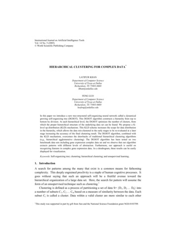
10L. Khan & F. Luo3.3.1.1. Average distortion (AD)AD is used to minimize intra-cluster distance. The average distortion of a sub tree with jchildren is defined as:ADj 1NN d (x , nii 1k)2(6)where O is the total number of input data assigned in the sub tree, and nk is the referencevector of the winner of input data xi. ADj is the average distance between input data andits winner. During DGSOT learning, the total distortion is already calculated and the ADmeasure is easily computed after the learning process is finished. If AD versus thenumber of clusters is plotted, the curve is monotonically decreasing. There will be amuch smaller drop after the number of clusters exceeds the “true” number of clusters,because once we have crossed this point we will be adding more clusters simply topartitions within rather than between “true” clusters. Figure 3(A) is an illustration of theaverage distortions versus the number of clusters. Figure 3(A) shows that after a certainpoint the curve becomes flat. This point indicates the optimal number of the clusters forthe sub-tree. Then, the AD can be used as a criterion for choosing the optimal number ofclusters. In the horizontal growth phase, if the relative value of AD after adding a newsibling is less than a threshold ε (Equation 7), then the new sibling will be deleted andhorizontal growth will stop.AD j 1 AD jADj ε(7)where j is the number of children in a sub-tree and ε is a small value, generally less than0.1.Figure 3. Illustration of AD Measure Versus Number of Clusters (A), and CS Measure Versus Number ofClusters (B).3.3.1.2. Cluster scatteringCluster scattering for determining the number of clusters can also be used in DGSOT.This measure minimizes the intra-cluster distance and maximizes inter-cluster distance.First, the minimum inter-cluster distance (MCD) is defined as:
Hierarchical Clustering for Complex DataMCD min( d(ni2– nj) )11(8)where d(ni – nj) is the distance between clusters i and j where i and j are the children ofthe same parent, and ni is the reference vector of node i. Then, the cluster scattering, CS,is defined as:AD(9)CS MCDTo determine the optimum number of children of a particular node, CS minimizes intracluster distances and maximizes inter-cluster distances. The number of clusters that givesthe first CS minimum value is taken to be the optimal number of clusters. Figure 3(B)illustrates the value of the CS measure versus the number of clusters. When the numberof clusters is small, the computational cost of CS is light. The advantage of using the CSmeasure is that it does not need a new threshold. But as a measure of validity, the CSmeasure tends to occur at the level of a smaller number of clusters than the valueobserved from the AD measure.4. Experimental ResultsIn this Section the DGSOT is applied to two datasets.4.1. Traditional data setFor the first set, we cluster two benchmark data sets from the UCI machine-learningrepository17: Wine. The Wine data represents 13 different chemical constituents of 178Italian wines derived from 3 different cultivars. The data of the Wine set is normalized tofacilitate the calculation of Euclidean distance. Wine dataset consists of three clusters.There are 178 data points and each data point has 13 attributes.A simple stopping rule is used to stop DGSOT from growing. A node in DGSOT willcease vertical growth if there is less than 10 data points. Both the AD and the CSmeasures have been used for horizontal growth. For the AD measure, ε is set to 0.05. αw,αs, αm. are set to 0.01, 0.001, 0.0005 respectively (see Section 3.2 for explanation). η(t)is set to 1/t where t is equal to 1 at the beginning; and in the next iteration of the learningit will be set to 2, and so on. K, TE and TH are set to 2, 0.001, and 10 respectively. Recallthat here heterogeneity of a leaf is determined based on the number of data associatedwith the leaf (see Section 3.1).The clustering result is displayed as a dendrogram. The data that belong to the samecluster will be in the same sub-tree. Figure 4 presents the clustering result of the Winedata. The letters A, B, C represent three kinds of wine. Figure 4(A) and 4(B) present theclustering result using the CS measure and the AD measure, respectively. The DGSOTdynamically finds the three clusters. The tree using the AD measure has more branches inhierarchy than the tree using the CS measure. Figure 4 shows that only 4 “B” class Winedata have been miss-clustered in both hierarchical trees. This result is better than that ofHAC, K-means and SOTA (see Table 2).
12L. Khan & F. LuoFigure 4. The DGSOT Clustering Result of the Wine Data Set. A) Using the CS Measure. B) Using the ADMeasure. (The letter A, B, C represents three kinds of wine respectively).Table 2. Compare clustering result on wine data.MethodNumber of miss-clustered dataHAC106K-Mean (K 3)7SOTA6DGSOT44.2. Complex data setSecond, we applied our hierarchical clustering algorithm to an existing 112 genesexpression data of rat central nervous system (CNS) reported and analyzed in Ref. 10.There are three major gene families among these 112 genes: Neuro-Glial Markers(NGMs), Neurotransmitter receptors (NTRs) and Peptide Signaling (PepS). All othergenes are considered by the author to constitute a fourth family called Diverse (Div).These gene expression data were measured by using RT-PCR in mRNA expression in ratcervica
benchmark data sets including gene expression complex data set and we observe that our algorithm extracts patterns with different levels of abstraction. Furthermore, our approach is useful on recognizing features in complex gene expression data. As a dendrogram, these results can be easily displayed for visualization.