WIXLIB

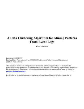
sterFigure 2: The data exploration pipeline for our system.2.2.2Interaction with the Clustering ProcessSystems that allow interaction with the clustering process are somewhat more rare. Many systems let users define initial cluster centroids in a visual way, rather than choosing them randomly. Thevalue of such a system, however, is unclear: if it is easy for the userto select centroids, it is probably unnecessary to cluster the data!Some systems go a bit further and allow the user to interact withthe clustering process as it is occurring. For example, Looney’swork [6] allows the user to eliminate or merge clusters at varioussteps in the algorithm. While this work takes strides to solve someof the major problems with clustering, it requires that the user understand the data set in order to produce a result. We seek exactlythe opposite paradigm: the user iteratively produces results in orderto understand the data set.2.2.3Alternatives to ClusteringSelf-organizing maps are an unsupervised learning technique builton neural networks. They have been widely explored as a tool toaid both visualization and data exploration [3, 4]. They are typically employed to aid in the production of low-dimensional visualizations of high-dimensional data.The benefits of self-organizing maps are somewhat contrary tothe goals of this work: they automatically reduce the dimensionality of the data, while providing little evidence of why a particularprojection was chosen. Instead, we enable the user to explore andre-weight dimensions at his or her discretion, helping the user tounderstand links between these dimensions.3DATA E XPLORATIONThe principle goal of our system is to enable intuitive data exploration of moderately-large, multi-dimensional data sets. In thispaper, we center our data exploration process around k-means, astraightforward clustering algorithm [7]. However, we believe ourdata exploration pipeline is applicable when coupling user interaction with any automated technique.We begin by explaining the difference between data explorationand data analysis. Then, we discuss our the details of our data exploration pipeline.3.1Data Exploration versus Data AnalysisThe distinction between data analysis and data exploration seemssubtle at first. Most simply, in data analysis, the user knows whathe or she is looking for; in data exploration, the user does not.Data analysis tasks typically investigate specific data instances,and their relation to other instances. The analyst usually has a largeunderstanding of the structure of the data set he or she is workingwith. That is, the relations between attributes are typically well understood, or at least the characteristics of a particular attribute arewell known. The examination of a gene array clustering, for example, is a typical data analysis task [1, 2]. The analyst knows whateach gene is, and what each experiment is, and is attempting todetermine which genes respond in similar ways to particular experiments. Such a task is completely static: a clustering is produced,visualized, and analyzed.Data exploration tasks are those which attempt to uncover thegeneral structure of the data. Here, the user may not know which attributes best separate or explain the data, may not know the relationships between attributes, and may not even know which attributesare useful. However, the user is likely to have domain knowledgeabout the data set being explored. For example, the user may havehigh-level knowledge about instances in the data set, and may beinterested in determining which attributes are most useful in predicting or explaining that knowledge.Data exploration is an iterative process of discovery. As such,tools for data exploration must support this iterative search. Specifically, we believe tools for data exploration must make it easy forthe user to explore the data along multiple paths, create branches in those exploration paths, and compare various exploration paths.3.2The Data Exploration PipelineThe use of our system centers around our Data ExplorationPipeline, shown in Figure 2.The user explores the data by iterating through this pipeline. After loading the data set, the user is presented with a visualization ofa solution to a trivial clustering problem: clustering all of the datainto one cluster. From this visualization, the exploration begins:1. The user explores a solution, visualizing it through the techniques described in Section 4.2. The user selects a subset of the data to continue exploring.This subset may, of course, be the entire set.3. The user generates a sub-problem using this subset of the data.This involves chooses the value of several parameters, suchas number of clusters to form, which attributes to use whenclustering, and the relative weights of each of those attributes.4. The clustering is performed and the sub-solution is stored.5. The process repeats using the new sub-solution.Of course, the user has more control over the pipeline than whatis given here. For example, the user can generate several differentsub-problems from any solution, varying the parameters (and eventhe sets) in each sub-problem. As a result of this flexibility, the

1Figure 3: A view of an individual cluster. The centroid is shown inred. The currently selected point is shown in blue. Points that lieclose to the selected point (in high-dimensional space) are shown ingray.pipeline results in a hierarchy of clustering solutions, where eachsub-solution is a refinement of a subset of its parent solution.Furthermore, as will be discussed in Section 4, we allow the userto open up visualizations of as many solutions as is desired, and linkthe display of these solutions so that similarities and differences caneasily be seen. In this way, it is easy for the user to explore theeffects of clustering using different features and parameters.When each solution is generated, we keep track of the parametersused in the clustering, as well as the parameters defining the subset of instances to be clustered. With this information, if new datais added to the system (for example, if we want to classify additional instances), we can place the new instances in the appropriateclusters in all solutions within the system.234Figure 4: Four views of the same centroid histogram. In each histogram, the centroid indicated is used as the basis.4.1.14V ISUALIZATION T ECHNIQUESIn this section, we examine the visualization techniques used tosupport the data exploration pipeline discussed in Section 3. Wedevote the majority of our attention to the techniques used to visualize a particular solution, and to compare several solutions, as thisis the novel portion of our system. However, in Section 4.2.1, wediscuss the interfaces for managing a hierarchy of solutions and forgenerating new solutions.The visualization techniques presented here have been developedwith the goals of effectively representing macro-level characteristics of clustering results and enabling intuitive comparison of multiple clustering solutions. These are the techniques required for dataexploration.While we provide some drill-down into the micro-level characteristics of a solution as a part of our brushing and highlightingtechniques, these characteristics are not our primary concern. Investigation of micro-level characteristics lies mainly in the domainof data analysis rather than data exploration. We believe that muchof the prior work discussed in Section 2 accomplishes the data analysis task successfully. So, in a complete system for both data exploration and analysis, we propose the marrying of our new techniqueswith extensions of existing analysis techniques. This is discussedfurther in our section on future work (Section 6.1).4.1Small Multiple Histograms for Cluster VisualizationIn the simplest sense, we visualize a clustering solution as a collection of histograms. Each cluster is represented by a histogram, asshown in Figure 3. The centroid of the cluster is placed on the leftof the histogram, and the instances are arranged according to theirEuclidean distance from the centroid. All of the histogram axes arescaled the same within one clustering solution. Complete sets ofsmall multiples for a solution can be seen in Figures 1 and 7.Centroid HistogramFurthermore, we produce a histogram layout of the centroids thatmimics the individual cluster histograms. The user is able to select the centroid to serve as the basis, and the other centroids areplaced in the histogram according to their Euclidean distance fromthe basis centroid. (This rocking of the basis element is discussedfurther in Section 4.1.3.) Examples of this visualization can be seenin Figure 4.Together, these histograms provide an intuitive summary ofmacro-level cluster characteristics. Cluster size and distributioncan easily be seen within one cluster histogram. Comparing clusterhistograms gives an understanding of relative compactness of eachcluster. Finally, the centroid histogram summarizes the inter-clusterseparation.4.1.2One Dimension versus Two DimensionsOur histograms can be thought of as a one-dimensional projectionof the data. At first consideration, it may seem that projecting intoone dimension (instead of two or three) gives up a great deal of flexibility. However, we believe that when combined with the decoupling of inter- and intra-cluster characteristics mentioned above, ourhistograms lead to a more faithful representation of the macro-levelcharacteristics than would be possible in a typical two-dimensionalprojection.Consider a projection of all instances into two dimensions usinga technique such as multi-dimensional scaling. In such a technique,one attempts to find the projection that preserves the pairwise distances between instances to the greatest extent possible. In mostcases, the actual distance between two points will be well reflectedby their distance in projected space. However, for some pairs ofinstances, such results may be impossible to achieve. It may bethat the best projection overall still places a significant number ofpoints close to other points that are actually far apart. Such misrepresentations make understanding macro-level characteristics of the

clustering result more difficult using this representation.Furthermore, even without these misrepresentations, the decoupling of inter- and intra-cluster characteristics in our method is noteasily achievable in a two-dimensional projection of all data. Instead, the user must segment the space mentally to perform suchcomparisons. Our decoupling allows the user to more easily examine the characteristics he or she is concerned about, without havingto block out additional information.As has been mentioned in Section 2, other two-dimensional techniques, such as colored matrix representations, exist for expressingcluster results. These techniques, however, are more suited towardmicro-level examination, which is outside the scope of this work.4.1.3RockingRocking is a technique often used to solve depth-cuing problemswhen visualizing three-dimensional point data in two dimensions.If the point set is rotated slightly, the necessary depth cue is provided: points in front move one direction while points in back movethe opposite direction.We borrow this idea of rocking to improve our histogram displays. In our histograms, it is often the case that two distant pointswill end up nearly the same distance from the centroid, and thus inthe same place on the histogram. (Note that this is not a misrepresentation, we make no claim that distant points will end up farapart in the histogram.) We allow the user to select two points, oneof which may be the centroid. After doing so, the first point is usedas the basis for computing distances to build the histogram. A slidercan be used to rock the basis point along the line between the firstand second points. As before, points that move left are closer tothe second point than the first, and conversely for points that moveright. An example of this is shown in Figure 5.As mentioned earlier, we allow a similar type of rocking withinthe centroid display. We allow the user to select a basis centroidby clicking. When the user changes basis centroids, new positionsfor each centroid in the histogram are computed, and the movementbetween old and new positions is animated. As before, the movements express the relative locations of other centroids as comparedto the two bases.Figure 4 shows all possible rockings of a single centroid histogram. From these views, it is clear that clusters 2 and 3 are located quite close to each other, whereas 1 and 4 are both far fromeach other and far from 2 and 3.4.2Data SubsettingA crucial part of the data exploration pipeline is the subsetting andreprocessing of data. We support data subsetting through dynamicqueries as shown in Figure 6. The user makes a range selectionsimply by dragging the range selection brackets so that they encloseonly the points of interest.Note that this range selection may be made with any point selected as the basis for distance calculation (and even when the basispoint is being rocked.) This allows the user to select points that areclose to (or far from) any point, rather than making selections withrespect to the centroid only.4.2.1Figure 5: Rocking of a cluster. The two points used to compute therocking line are shown in yellow. The amount of rocking is controlledby moving the slider.Generating Solution HierarchiesOnce the desired subset is selected within each cluster histogram,a new sub-solution may be generated. The Sub-Solution Generatorwindow (not shown) presents a simple user interface to select theattributes for clustering, assign weights to those attributes, choosethe number of clusters to be formed, and initiate the clustering.When a new clustering solution is generated, it is placed in theSolution Explorer (shown in Figure 1) as a child of its parent solution. Any number of child and grandchild solutions may be createdFigure 6: A dynamic query within a cluster histogram, used for bothdata subsetting and range selection in view linking.

from any parent solution. In this way, the user is able to traversemultiple exploration paths, branching as desired. The Solution Explorer keeps each solution organized, providing a summary of theattributes used to generate the clustering.4.3Brushing and View LinkingWith the generation of multiple solutions comes the need to explorethem in concert. We support this exploration through brushing andview linking.As shown in Figure 3, brushing is used to highlight instancesnear a selected instance (in high-dimensional space). When a userhovers over an instance, it is highlighted in blue. Additionally, allnearby instances are colored gray. Note that this highlighting issomewhat akin to rocking. Only the instances which are actuallynear the instance of interest are highlighted. In addition to highlighting close-by instances within the cluster, we also highlight instances corresponding to the selected instance in all other views.Similarly, we highlight all instances contained within the activeregion of the currently selected cluster in all solution visualizations.(The currently selected cluster is defined by the chosen basis centroid in the currently focused window.) This highlighting is shownin Figure 7.View linking allows the user to easily visualize the relative consistency of clustering between different solutions using different attributes and weights. In this way, relations between attributes can beeasily found and understood, helping the user uncover the structureof the data, the ultimate goal of data exploration.4.4Micro-level Data ExaminationA minimal amount of support is provided within the system formicro-level data examination. The member table, shown in Figure 1, lists all instances in the currently selected cluster. Brushingis supported between the member table and solution visualization:the selected instance in the visualization is highlighted in the member table, and likewise, a selected instance in the member table ishighlighted in the solution visualization. Finally, if a range selection is made within the active cluster, only the selected instancesare shown in the member table.Support for micro-level data examination could be greatly enhanced by building upon much of the prior work mentioned in Section 2.1.1. We discuss our plans for this further in Section 6.1. Nonethe less, we believe that the linking of brushing between macro- andmicro-level visualizations presented here here would prove to be avery useful feature regardless of the micro-level visualization used.5E XAMPLE U SEIn this section, we present a brief example of one possible use ofour system. Consider a network administrator who is attemptingto locate machines that are behaving atypically. The administratorbelieves that the usage patterns of most machines stay consistentfrom month to month, and that a change in behavior might be anindication of an intrusion or other exploit. However, she has a largenumber of traffic metrics available to her, and is not sure which ofthese metrics best express a machine’s usage pattern.The network administrator begins her data exploration by compiling a variety of traffic metrics for each month for each machine.Each of these values becomes an attribute. Each instance (a machine) has a group of attributes for each month of data, resulting inn · m attributes, where n is the number of traffic metrics, and m isthe number of months. All of this data is loaded into the system.She first decides to cluster the entire dataset into 5 clusters using the all of the first months attributes. To do this, she opens theinitial solution (a clustering of everything into one cluster) presentin the Solution Explorer. She does not need to subset the data, soshe simply uses the Sub-Problem Generator to define her clusteringproblem: she selects the attributes of interest and chooses 5 clusters.After the clustering is completed, she visualizes the new solution. She observes that two clusters contain most of the instances.She quickly hovers over the few instances that lie in the other threeclusters. She discovers that all of these machines are servers of onesort or another. Since she watches these machines pretty closely using other tools, she decides to exclude them from her exploration.She makes an empty range selection in each of these clusters, leavesthe entire range selected in the two dense clusters, and opens up theSub-Problem Generator again.She decides now to try to confirm her theory that the behavior ofmost machines does not change from month to month. Using thesubset of machines selected, she produces two new sub-solutions:one using the first month’s attributes, and one using the secondmonth’s attributes. She opens up both solutions, and utilizes theview linking features to explore their similarity. This explorationis shown in Figure 7. She selects each cluster in the first month’svisualization in turn. As she does so, the corresponding instancesin the second month’s visualization are highlighted. As is shownin Figure 7, the clusters stay relatively consistent. She quickly examines those instances that change clusters. For some, she easilyobserves that the machines are outliers in both clustering solutions.This suggests that the attributes or weights in use may not be optimal. For others, she uses her domain knowledge to explain thedifferences. For example, perhaps one of the instances is a machinethat was added in the middle of the first month. For a few others,she decides to do further investigation.From this point, her data exploration process could go any number of directions. She could produce several clustering solutions forthe same month using different attributes to explore links betweenthe attributes. She could produce clustering solutions of varyingsizes for the same attributes, giving her a clearer picture of howmany types of machines she really has. The system easily supportsthese and many other tasks. Furthermore, once she has determinedthe set of attributes and weights that best characterizes her data, shecan carry this information over into the data analysis domain anduse these same clustering techniques in her daily network monitoring.6C ONCLUSIONWe have presented a visualization system that harnesses clustering algorithms to make exploration of moderately-large, highdimensional data sets more intuitive. An iterative process of visualization, query refinement, and re-processing was presented thatwe believe accurately represents the ideal data exploration process.Furthermore, we proposed a novel method for visualizing macrolevel clustering characteristics. Finally, we showed an example useof our system.6.1Future WorkWe believe that a complete solution would provide means for bothdata exploration and data analysis. In this work, we have only explored the domain of data exploration. We are interested in augmenting the visualizations presented here with adaptations of someof the techniques presented in Section 2 to produce such a completesystem.We also plan to characterize more clearly the trade-offs betweenexisting two-dimensional visualizations and the one-dimensionalapproach

ally center around hiding data. When hierarchical clustering is performed, visualization tools often provide a means for collapsing portions of the hierarchy. The Hierarchical Clustering Explorer [10] supports this through dynamic queries, and gCLUTO [9] supports this through a typi-cal expandable tree structure. While these methods are .