WIXLIB

Figure 1: A hierarchical Time dimension. A hierarchical dimension is structured as a tree with multiple levels. In this case, there are fourlevels: All, Year, Quarter, and Month. Each level corresponds to a different semantic level of detail. The parent-child relationships in the treeare the basis for aggregation within the dimension.data) and to brush records based on their proximity within the hierarchical structure. Again, this approach limits the user, in this caseto viewing a single hierarchical structuring of the data and a singleordering of that hierarchy to make proximity meaningful. Polarissupports both the simultaneous exploration of multiple hierarchies(derived from semantic meaning or algorithmic analysis) and theability to reorder the hierarchy as needed.Another relevant database visualization system is VisDB [12],which focuses on displaying as many data items as possible to provide feedback as users refine their queries. This system even displays tuples that do not satisfy the query, indicating their “distance”from the query criteria using spatial encodings and color. This approach helps the user avoid missing important data points that falljust outside of the selected query parameters. In contrast, Polaris,by taking advantage of the hierarchical structure of the warehouse,provides extensive ability to drill down and roll up data, allowingthe analyst to get a complete overview of the data set before focusing on detailed portions of the database.2.2Visualization and Data MiningMany research and commercial systems use visualization in conjunction with automated data mining algorithms. One common application of visualization together with data mining is in helpinganalysts understand models generated by the data mining process.For example, several researchers have developed techniques specifically for displaying decision trees, Bayesian classifiers, and decision table classifiers [1], and these visualization techniques havebeen incorporated into products such as SGI’s MineSet [3].Other approaches to coupling visualization and data mining havetraditionally been employed within focused domains. One approach is to use visualization to gain an initial understanding ofa warehouse and then apply algorithmic analysis to the identifiedareas of interest [13][22]. The other major approach is to use datamining to compress the size and dimensionality of the data and thenuse focused visualization tools to explore the results [10][25].Unlike these examples, Polaris is not focused on a particular algorithm, a single phase of the discovery process, or a narrow application domain. Instead, Polaris is a general tool that can be usedto gain an initial understanding of a warehouse, to visually minethe warehouse, to understand algorithm output, and to interactivelyexplore a mining model. The ability to encode a large number ofdimensions in a table layout in Polaris helps an analyst gain an initial understanding of how different dimensions relate as a precursorto automated discovery. Similarly, Polaris can be used directly asa visual mining tool. Finally, by integrating the decision trees andclassification networks into the data warehouse as dimensional hierarchies, Polaris can be used by analysts to gain an understandingof how these models classify the data.3BackgroundPolaris [20] was originally designed to support the interactive exploration of multidimensional relational data warehouses ratherthan data sets with rich hierarchical structure. In this section, weexplain the difference between the two types of data sources as wellas give a brief overview of Polaris before discussing our extensionsto Polaris in the rest of the paper.3.1Relational Databases vs. Data CubesRelational databases organize data into relations, where each rowin a relation corresponds to a basic entity or fact and each columnrepresents a property of that entity [23]. For example, a relationmay represent transactions in a bank, where each row correspondsto a single transaction, and each transaction has multiple properties,such as the transaction amount transaction, the account balance, thebank branch, and the customer.We refer to a row in a relation as a tuple or record, and a columnin the relation as a field. A single relational database will containmany heterogeneous but interrelated relations.The fields within a relation can be partitioned into two types:dimensions and measures. Dimensions and measures are similarto independent and dependent variables in traditional analysis. Forexample, the bank branch and the customer would be dimensions,while the account balance would be a measure.In many data warehouses, these multidimensional databases arestructured as n-dimensional data cubes. Each dimension in thedata cube corresponds to one dimension in the relational schema.Each cell in the data cube contains all the measures in the relationalschema corresponding to a unique combination of values for eachdimension.The dimensions within a data cube are often augmented witha hierarchical structure. This hierarchical structure may be derivedfrom the semantic levels of detail within the dimension or generatedfrom classification algorithms. Using these hierarchies, the analystcan explore and analyze the data cube at multiple meaningful levelsof aggregation calculated from a base fact table (i.e., a relation inthe database with the raw data). Each cell in the data cube nowcorresponds to the measures of the base fact table aggregated to theproper level of detail.The aggregation levels are determined from the hierarchical dimension, which is structured as a tree with multiple levels. Eachlevel corresponds to a different semantic level of detail for that dimension. Within each level of the tree there are many nodes, witheach node corresponding to a value within the domain of that levelof detail of that dimension. The tree forms a set of parent-child relationships between the domain values at each level of detail. Theserelationships are the basis for aggregation, drill down, and roll upoperations within the dimension hierarchy. Figure 1 illustrates thedimension hierarchy for a Time dimension.Simple hierarchies, like the one shown in Figure 1, are commonly modeled using a star schema. The entire dimensional hierarchy is represented by a single dimension table (also stored as arelation) joined to the base fact table. In this type of hierarchy, thereis only one path of aggregation. However, there are more complexdimension hierarchies where the aggregation path can branch. For

Figure 2: The Polaris user interface with enhancements (shown in blue) to expose and support hierarchical dimensions. Analysts constructtable-based displays of relational and cube data by dragging dimension levels and measures from the data cube schema onto shelves throughout the display. A given configuration of levels and measures on shelves is called a visual specification. The specification unambiguouslydefines the analysis and visualization operations to be performed by the system to generate the display.example, a Time dimension might aggregate from Day to both Weekand Month. These complex hierarchies are typically represented using a snowflake schema that uses multiple relations to represent thediverging hierarchies.When referring to values within a dimension hierarchy, we willuse a dotted notation to specify a specific path from the root level(All) of the hierarchy down to the specified value. Specifically, torefer to a value on level m of a hierarchy, we first optionally listthe dimension name, then zero or more of the (m 1) intermediateancestor values, and then finally the value on the mth level, allseparated by periods. For example, the Jan node on the Monthlevel in the Time hierarchy that corresponds to January, 1998, canbe referred to as 1998.Qtr1.Jan. When this notation is used, wewill call the reference a qualified value. When a value is simplydescribed by its node value (without any path to the root node) wecall the reference an unqualified value.3.2Polaris OverviewBefore explaining the extensions to Polaris needed for supportinginteractive visual exploration of hierarchically structured data sets,we first give a brief overview of the original Polaris system.The goal of Polaris was to provide an interface for rapidly andincrementally generating table-based displays (note that from hereon out, unless otherwise specified as a fact table or dimension table,the term table refers to a table-based visualization and not a relationin a database). Users construct these table-based visualizations viaa drag-and-drop interface, dragging field names from the Schemabox to various blue shelves throughout the interface, as shown inFigure 2. Any configuration of field names on shelves is valid.The Polaris interface is simple and expressive because it is builtupon a formalism for precisely describing graphical table-based visualizations. The configuration of fields on shelves forms a visualspecification. Each visual specification is an expression of the Polaris formalism that can be interpreted to determine the exact analysis, query, and drawing operations to be performed by the system.The specification consists of two main portions. The first portion, built on top of an algebra, describes the structure of the tablebased visualization (i.e., how the table is divided into panes). Wecan think of a table as having three axes: the x-axis divides the tableinto columns, the y-axis divides the table into rows, and the z-axislayers x-y tables that are composited on top of one another. Eachintersection of an x, y, and z axis results in a table pane. Thus,the first portion of the specification consists of table algebra expressions, with one expression per axis. Each pane contains a setof records (obtained by querying the data cube) that are visuallyencoded as a set of marks to create a graphic.While the first portion of the specification determines the “outertable layout,” the remaining portion determines the layout within apane, such as how the data within a pane is transformed for analysisand how it is encoded visually. Specifically, it describes:1. The sorting and filtering of fields.2. The mapping of data sources to layers.3. The grouping of data within a pane and the computation ofstatistical properties, aggregates, and other derived fields.4. The type of graphic displayed in each pane of the table. Eachgraphic consists of a set of marks (e.g., circles, bars, glyphs,etc.), with one mark per record in that pane.5. The mapping of data fields to retinal properties of the marksin the graphics (for example, mapping Profit to the size of amark or Quarter to the color).

Figure 3: Example of the set interpretations and table structures resulting from simple applications of the table algebra operators. Ordinalfields (e.g., dimension levels) partition the table into columns (or rows) and quantitative fields (e.g., measures) are spatially encoded as axeswithin the columns. Note the difference between the application of the nest and dot operator to the same operands when the fact table doesnot contain data for October.We only need to extend the table algebra and the specification ofthe filtering and sorting. The rest of the formalism, including howwe determine the type of graphic and the visual encodings, has notchanged and so we do not discuss them further here. See Stolte etal. [20] for a detailed discussion.Thus, in order to extend Polaris to support hierarchical dimensions, we need to modify: the formalism and table algebra (described in Section 4) the user interface (described in Section 5) and the interpretation of the visual specification as a set ofqueries in a multidimensional query language (described inSection 6).4Extending the FormalismIn order to support both relational databases and hierarchicallystructured data cubes, we need to extend two aspects of the Polarisformalism: the specification of the table configurations, and the filtering and sorting of fields. Before we discuss these two extensions,however, we first give a brief review of the table algebra.4.1Table Algebra ReviewA key component of this formalism is the table algebra, which isused to specify the table configurations. When analysts place fieldson the axis shelves (shown in Figure 2) they are implicitly creatingexpressions in this algebra. A complete table configuration consistsof three separate expressions. Two of the expressions define theconfiguration of the x and y axes of the table, partitioning the tableinto rows and columns. The third expression defines the z axis ofthe table, which partitions the display into layers.Each expression is composed of operands connected by operators. Each operand is evaluated to a set form, and the operatorsdefine how to combine two sets. Thus, each expression can be interpreted as a single set (the normalized set form), where each elementin the set corresponds to a single row, column, or layer.To be more specific, each operand of the table algebra is thename of a field. There are two types of operands: ordinal and quantitative. Whether an operand is ordinal or quantitative depends onthe type of the corresponding field in the database.The set interpretation of an ordinal operand consists of the members of the ordered domain of the field. For example, the set interpretation of the Month operand would be {Jan, Feb, . . . , Dec}. Theset interpretation of a quantitative operand is a single-element setcontaining the field name. For example, the set interpretation of theProfit operand would be {Profit}.The assignment of sets to the different types of operands reflectsthe difference in how the two types of fields are encoded into thestructure of the table. Ordinal fields partition the table into rowsand columns, whereas quantitative fields are spatially encoded asaxes within the table panes. Examples of the set interpretations andresulting table structures for both ordinal and quantitative operandsare shown in Figure 3.As stated above, a valid expression in the algebra is an orderedsequence of one or more operands with operators between each pairof adjacent operands. The operators in this algebra, in order ofprecedence, are cross ( ), nest (/), and concatenation ( ); paren-

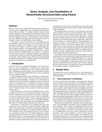
Figure 4: Each pane in a Polaris visualization corresponds to a slice of a projection of a data cube. The projection in each pane is determinedby the contents of the “Level of Detail” shelf and by the normalized set form of the table expressions. The table is partitioned into rows,columns, and layers corresponding to the entries in these sets. The underlying data cube must be projected to include only the dimensionsthat occur in these entries. This is shown here for a simple text-based table. Generating this table requires two separate projections of the datacube because of the concatentation in the y-axis expression.theses can be used to alter the precedence. Because each operand isinterpreted as an ordered set, the precise semantics of each operatorare defined in terms of how they combine two sets (one each fromthe left and right operands) into a single set. Some examples areshown in Figure 3.Thus, every expression in the algebra can be reduced to a singleset, with each entry in the set being an ordered concatenation ofzero or more ordinal values followed by zero or more quantitativefield names. For example, the normalized set form of the expressionMonth Profit is { (Jan, Profit), (Feb, Profit), . . . , (Dec, Profit) }.The normalized set form of an expression determines one axis of thetable: the table axis is partitioned into columns (or rows or layers)so that there is a one-to-one correspondence between columns andentries in the normalized set.4.2Redefining the Algebra OperandsIn order to fully support and expose the hierarchical structure indata cube dimensions, we must redefine the algebra so that theoperands are measures and dimension levels rather than independent database fields. In this redefinition, measure operands are trivially treated the same as quantitative fields: we assign to each measure operand a single element set containing the measure name.Like quantitative fields in the original algebra, measures will bespatially encoded as axes within the panes.Similarly, we would like to treat dimension levels in the sameway we treated ordinal fields and assign to each the ordered domainof the dimension level. The resulting sets would then partition thetable into rows, columns, and layers. There are, however, complications. The domain of a dimension level is not a single ordered list.Instead, it is composed of the node values at a particular level in thedimension hierarchy, and each node value is uniquely defined by itspath to the root of the hierarchy. To illustrate the complications thiscauses, we consider the Time hierarchy illustrated in Figure 1.First, consider the Month level of the hierarchy. One possibleset interpretation of this symbol would be to list each node value,including its path to the root for uniqueness, ordered by a depthfirst traversal of the dimension hierarchy; e.g., {1998.Qtr1.Jan,. . . , 1999.Qtr4.Dec}. Although this approach provides a uniqueset interpretation for each dimension level, it limits the expressiveness of the algebra. Any table constructed to include Month mustalso include Year; it is not possible to create displays that summarize monthly values across years, a useful view that we wouldlike to support. Interestingly, however, summarizing monthly values across years is not a standard projection of a data cube, as itrequires aggregating across a hierarchical level. We discuss howthis type of aggregation is computed in Section 6.A second approach would be to list only the node values, ignoring the path to the root of the hierarchy and excluding repeated values. Again, we order the node values by a depth-first traversal of thedimension hierarchy. For Month, this would yield {Jan, Feb, . . . ,Nov, Dec}. Clearly, using this set interpretation we can generatedisplays that summarize monthly values across years. Furthermore,we can generate displays that drill down into a hierarchy by usingour nest (“/”) operator; e.g., Year / Month.The use of the nest for drilling down into a hierarchy, however,would be flawed. The nest operator is unaware of the defined hierarchical relationship between the dimension levels but instead worksby deriving a relationship based on the tuples in the fact table. Notonly is this inefficient, as fact tables are often quite large, but itcan also yield incorrect results. For example, consider the situationwhere no data was logged for October. Application of the nest operator would result in an incorrectly derived Time hierarchy that didnot include October as a child of Qtr4 or either year (see Figure 3).Our solution is to introduce another operator, the dot (“.”) operator, that is similar to the nest operator but “hierarchy-aware.” Wereview the definition of nest and then define dot. If we define FT tobe the fact table being analyzed, r to be a record, and A(r) to be thevalue of the field A for the record r, then the definition of nest, aspresented in [20], is:A/B {(a, b) r F T st A(r) a & B(r) b}The dot operator is defined similarly. If we define DT to be therelational dimension table defining the hierarchy that contains thelevels A and B, and A precedes B in the schema of DT, then:A.B {(a.b) r DT st A(r) a & B(r) b}Note that whereas nest produces a set of two-valued tuples, dotproduces a set of single-valued tuples, each containing a qualifiedvalue. If the two operands are not levels of the same dimensionhierarchy (or set interpretations of operations on levels of the samehierarchy), or A does not precede B in the schema of DT (e.g., Amust be an ancestor level in the tree defined by DT) , then the dotoperator evaluates to the empty set. With this definition, the twoexpressions Month and Year.Month are not equivalent: Month isinterpreted as {Jan, Feb, . . . , Dec} whereas Year.Month would beinterpreted as {1998.Jan, 1998.Feb, . . . , 1999.Dec}. With a fullypopulated fact table, Year.Month is equivalent to Year / Month.Given these set interpretations for dimension and measureoperands, we can apply the set semantics for each operator to reduce expressions in this new algebra to their normalized set form,

with each entry in the normalized set being an ordered concatenation of zero or more domain values followed by zero or moremeasure names. As before, the normalized set form determines oneaxis of the table.4.3Filtering and Sorting within the AlgebraIn our original formalism, a table configuration was specified bythree expressions in the table algebra, and then filtering and sortingwas specified separately by listing the sorted and filtered domainfor each database field that was to be filtered or sorted. When theset interpretation was generated for field operands in the algebra,these specified domains would be used. It is possible, however, togenerate a more succinct and general formalism if we incorporatethe filtering and sorting directly into the table algebra.In our revised formalism, if a dimension or measure is to be filtered (or sorted), then the filtered and sorted domain is listed directly after the instance of the level or measure operand in the expression, in effect directly specifying a set interpretation for theoperand. For example, if we wished to filter the expression Month ProductType to include only the first three months of the year,sorted in reverse order, this could be specified by including the filtered domain in the expression as follows: Month{Mar, Feb, Jan} ProductType. The advantage provided by this revision of the table algebra is the ability to specify separate filters and orderingsfor different instances of the same operand in an expression. Similarly, we can filter a measure by specifying a range of values, e.g.,Profit{0, 500}.We also need to allow the use of qualified values in the specification of filtering or sorting of dimension levels. As we discussed in Section 3.1, a value in a dimension hierarchy can eitherbe described by simply stating the value in the node (an unqualified value) or by describing a path from that node to the root nodein the hierarchy (a qualified value). When filtering or sorting a dimension level, it is necessary to be able to use both types of valuesin the specification, as the unqualified node values are often notunique. For example, if the user wishes to exclude 1998.Jan but not1999.Jan, then qualified values must be used.5Redefining the User InterfaceHaving redefined the formalism underlying the Polaris interface,we must now alter the interface to support hierarchically structureddata. Five major changes need to be made:1. the Schema list must display dimension hierarchies and measures, not simply database fields;2. the analyst must be able to distinguish between Month andYear.Month when including Month in a specification;3. the analyst must be able to filter a dimension level using qualified values;4. the analyst must be able

structured data via three case studies (Section 7). 2 Related Work We consider two areas of related work: the visual exploration of databases and the use of data visualization in conjunction with data mining algorithms. 2.1 Visual Exploration of Databases One area of related work is the field of visual query tools. Projects