Transcription
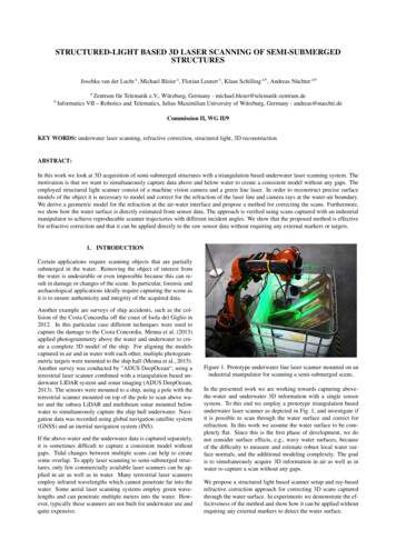
STRUCTURED-LIGHT BASED 3D LASER SCANNING OF SEMI-SUBMERGEDSTRUCTURESJoschka van der Lucht a , Michael Bleier a , Florian Leutert a , Klaus Schilling a,b , Andreas Nüchter a,babZentrum für Telematik e.V., Würzburg, Germany - michael.bleier@telematik-zentrum.deInformatics VII – Robotics and Telematics, Julius Maximilian University of Würzburg, Germany - andreas@nuechti.deCommission II, WG II/9KEY WORDS: underwater laser scanning, refractive correction, structured light, 3D reconstructionABSTRACT:In this work we look at 3D acquisition of semi-submerged structures with a triangulation based underwater laser scanning system. Themotivation is that we want to simultaneously capture data above and below water to create a consistent model without any gaps. Theemployed structured light scanner consist of a machine vision camera and a green line laser. In order to reconstruct precise surfacemodels of the object it is necessary to model and correct for the refraction of the laser line and camera rays at the water-air boundary.We derive a geometric model for the refraction at the air-water interface and propose a method for correcting the scans. Furthermore,we show how the water surface is directly estimated from sensor data. The approach is verified using scans captured with an industrialmanipulator to achieve reproducable scanner trajectories with different incident angles. We show that the proposed method is effectivefor refractive correction and that it can be applied directly to the raw sensor data without requiring any external markers or targets.1. INTRODUCTIONCertain applications require scanning objects that are partiallysubmerged in the water. Removing the object of interest fromthe water is undesirable or even impossible because this can result in damage or changes of the scene. In particular, forensic andarchaeological applications ideally require capturing the scene asit is to ensure authenticity and integrity of the acquired data.Another example are surveys of ship accidents, such as the collision of the Costa Concordia off the coast of Isola del Giglio in2012. In this particular case different techniques were used tocapture the damage to the Costa Concordia. Menna et al. (2013)applied photogrammetry above the water and underwater to create a complete 3D model of the ship. For aligning the modelscaptured in air and in water with each other, multiple photogrammetric targets were mounted to the ship hull (Menna et al., 2015).Another survey was conducted by ”ADUS DeepOcean“, using aterrestrial laser scanner combined with a triangulation based underwater LIDAR system and sonar imaging (ADUS DeepOcean,2013). The sensors were mounted to a ship, using a pole with theterrestrial scanner mounted on top of the pole to scan above water and the subsea LiDAR and multibeam sonar mounted belowwater to simultaneously capture the ship hull underwater. Navigation data was recorded using global navigation satellite system(GNSS) and an inertial navigation system (INS).If the above-water and the underwater data is captured separately,it is sometimes difficult to capture a consistent model withoutgaps. Tidal changes between multiple scans can help to createsome overlap. To apply laser scanning to semi-submerged structures, only few commercially available laser scanners can be applied in air as well as in water. Many terrestrial laser scannersemploy infrared wavelengths which cannot penetrate far into thewater. Some aerial laser scanning systems employ green wavelengths and can penetrate multiple meters into the water. However, typically these scanners are not built for underwater use andquite expensive.Figure 1. Prototype underwater line laser scanner mounted on anindustrial manipulator for scanning a semi-submerged scene.In the presented work we are working towards capturing abovethe-water and underwater 3D information with a single sensorsystem. To this end we employ a prototype triangulation basedunderwater laser scanner as depicted in Fig. 1, and investigate ifit is possible to scan through the water surface and correct forrefraction. In this work we assume the water surface to be completely flat. Since this is the first phase of development, we donot consider surface effects, e.g., wavy water surfaces, becauseof the difficulty to measure and estimate robust local water surface normals, and the additional modeling complexity. The goalis to simultaneously acquire 3D information in air as well as inwater to capture a scan without any gaps.We propose a structured light based scanner setup and ray-basedrefractive correction approach for correcting 3D scans capturedthrough the water surface. In experiments we demonstrate the effectiveness of the method and show how it can be applied withoutrequiring any external markers to detect the water surface.
2. RELATED WORKCorrection of optical measurements through the water surfacehas been studied for various applications of laser scanning andphotogrammetry, e.g, airborne laser scanning of coast lines (Hilldale and Raff, 2008; Wang and Philpot, 2007; Irish and Lillycrop,1999; Saylam et al., 2017) or sunken archeological sites (Doneuset al., 2013), photogrammetric measurements of river beds (Westaway et al., 2003) or convection flow estimation in a glass vessel (Maas, 2015).Narasimhan and Nayar (2005) investigated the application of lightstripe projection and photogrammetric stereo on multimedia scanning. They employ a camera-projector setup in air that measuresobjects in a water tank. To correct for the refraction at the transition between air and water the refraction of the camera ray aswell as the projector ray need to be considered. For calibrationtwo planes at known distance are placed in the water tank. Moreover, they studied the effects of scattering media by adding milkto the water and developed a method to correct the color of thescans.Klopfer et al. (2017) apply a Microsoft Kinect RGB-D camerato capture bathymetry with the sensor placed above the water.Although the infrared pattern projector of the Kinect suffers fromhigh absorption in water, measurements at depths of up to 40cmwere achieved. The sensor was mounted parallel to the watersurface and the distance between the water plane and the sensorwas measured. The point clouds captured by the Kinect were thencorrected based on a ray-based refraction model.The work of Palomer et al. (2017) does not concern itself withscanning in the water with a sensor in air, but the refraction correction necessary for their underwater laser scanner is similar.Since a mirror galvanometer-based laser projector is employed toproject different laser lines in the underwater environment, theincident angles of the laser rays differ from each other. Instead ofusing a ray-based correction model Palomer et al. (2017) modelthe deformed laser plane with a pyramid cone. To reconstruct thelaser points, the camera rays are intersected with the calibratedmodel of the deformed planes.Some of the published literature also addresses inaccuracies introduced by waves, which are very difficult to model exactly. Inearly work Okamoto (1982) studied the influence of waves onaerial imaging of shallow waters. Fryer and Kniest (1985) examined the resulting errors for the application of stereo vision forcreating digital elevation maps of shallow waters from an aerialplatform. To achieve structured light imaging through a wavy water interface Sarafraz and Haus (2016) use a calibration target foronline estimation of the water surface. In their setup a calibratedprojector-camera setup is employed with the projector in air andthe camera placed in the water. The scene is illuminated witha dot pattern. Underwater the camera observes the shift of theprojected pattern on a checkerboard target. From this observation a model of the water surface is estimated. Objects placed onthe same plane as the calibration target can then be reconstructedby computing the refraction for all observed projector rays. Therestriction of this method is that it can be applied only to a controlled environment because the water surface is assumed to bemodeled by a combination of sinusoidal functions.3. METHODOLOGYIn this work we employ a triangulation based line laser scanner.To create a precise point cloud of a semi-submerged scene weFigure 2. Prototype structured light underwater scannerprojecting a laser cross in a water tank.first scan the scene and create a 3D reconstruction without considering the refraction at the water interface. Since the employedstructured light scanner captures only a profile, we need to movethe scanner to create a complete 3D scan of the scene. We capture and record the 6-DOF movement of the scanner system externally. Then, from the sensor data we extract the water surface andcorrect all 3D point measurements inside the water body using aray-based approach. In this section we describe the employedscanner hardware, how we calibrate the scanner, the 3D reconstruction approach and how the refraction at the water interfaceis modeled and corrected.3.1 Underwater Laser ScannerThe employed underwater 3D cross line laser scanner consists oftwo housings, one containing the camera and the other one thecross line laser projector. For the experiments in this work weemploy a baseline of approximately 40 cm between the cameraprojection center and the laser plane. The laser plane inclinationof the scanner is 20 deg. Both housings include an inertial measurement unit (IMU) and an embedded PC with network interface. The two housings are mounted on a 0.5 m long aluminumbar. The camera housing is mounted at an angle of 30 to the bar.The system is depicted in Fig. 2. For the experiments in this workonly one of the two laser lines of the cross laser projector is used.Fig. 3 shows a cross-section of the camera housing and the laserhousing. The camera housing, which is depicted in the top imagein Fig. 3, includes the lens with a focal length of 12.5 mm (labeled (a)). The camera is a FLIR Blackfly 2.3 Megapixel colorFigure 3. Cross-sections of the CAD models: the top imageshows the camera housing and the bottom image shows thehousing of the cross line laser projector.
do not have to consider the distortion parameters during the 3Dreconstruction step, which simplifies the equations presented inthe following sections.For calibrating the laser projector it is necessary to determine thelaser plane parameters relative to the origin of the camera coordinate system. To do this, a L-shaped 3D calibration pattern, depicted in Fig. 4, consisting of two planes with AprilTags is used.This enables determining the laser plane equation from a singleimage.Figure 4. Calibration of the laser plane parameters using aL-shaped calibration target.camera (labeled (b)) with a 1/1.2” Sony Pregius IMX249 CMOSsensor. The image resolution is 1920 1200 pixels with 5.86 µmpixel size and a maximum framerate of 41 fps. An IMU (labeled(c)) is centered above the camera. For image processing an embedded PC (labeled (d)) is included in the housing.The bottom image in Fig. 3 shows the components of the laserhousing. The laser projector is constructed from Powell laserline optics (labeled (a)), beam correction prisms (labeled (b))and the laser diodes (labeled (c)) The lasers are two 1 W greendiode lasers with a wavelength of 525 nm, which are controlledby power and control electronics (labeled (d)) and connected toan embedded PC (labeled (e)). A second IMU (labeled (f)) is installed for orientation determination. The two laser lines projecta laser cross consisting of two perpendicular lines in the scene.The lasers can be fired synchronized to the camera shutter usingtrigger signals.3.2First, we detect the L-shaped pattern in the camera image andcompute the pose relative to the calibrated camera. From thiswe can compute the parameters of the two individual planes ofthe calibration target. Then, we detect laser points lying on thetwo calibration planes and reconstruct their 3D position by intersecting the camera ray with the respective calibration plane. Theplane parameters of the laser plane can then be found by fitting aplane to the the reconstructed 3D laser point positions. We compute the best fitting plane based on a robust fit using RANSACover multiple calibration images to improve the final solution.3.3 3D ReconstructionOnce we have calibrated the system and know the camera modeland laser plane parameters 3D reconstruction is performed usinglight section by intersecting the camera rays with the laser plane.We describe the laser plane πi using the general formπi :CalibrationWe approximate the camera projection function based on the standard pinhole model with distortion. The point X (X, Y, Z)Tin world coordinates is projected on the image plane according to(X, Y, Z)T 7 (fxXY px , fy py )T (x, y)T , (1)ZZwhere x (x, y)T are the image coordinates of the projection,p (px , py )T is the principal point and fx , fy are the respectivefocal lengths. We use separate focal lengths instead of a singleprincipal distance in order to absorb small modeling inaccuracies. However, in our particular case the difference between theestimates for fx and fy is small.Using the normalized pinhole projection X/Zxn xn Y /Zynai X bi Y ci Z 1 ,where (ai , bi , ci ) are the plane parameters and X (X, Y, Z)Tis a point in world coordinates. Using the perspective cameramodel described in Eq. 1 this is expressed asπi :aix px1y py bi ci ,fxfyZwe include radial and tangential distortion defined as follows x̃ xn 1 k1 r 2 k2 r 4 k5 r 6 (3)2k3 xn yn k4 (r 2 2x2n ), 22k3 (r 2yn ) 2k4 xn ynwhere (k1 , k2 , k5 ) are the radial and (k3 , k4 ) are the tangentialdistortion parameters. Here, x̃ (x̃, ỹ) are the real (distorted)normalized point coordinates and r 2 x2n yn2 .We calibrate the camera using Zhang’s method (Zhang, 2000)with a 3D calibration fixture with AprilTags (Olson, 2011) asfiducial markers. The advantage here is that calibration points areextracted automatically even if only part of the structure is visiblein the image. After performing laser line extraction we undistortall image coordinates of the detected line points. Therefore, we(5)where x (x, y)T are the image coordinates of the projection ofX on the image plane, p (px , py )T is the principal point andfx , fy are the respective focal lengths.The coordinates of a 3D object point X (X, Y, Z)T on theplane from its projection on the image plane x (x, y)T can becomputed by intersecting the camera ray with the laser plane:Z (2)(4)1y pyx b ciai x pi ffxyx pxfxy pyY Z.fyX Z(6)3.4 Estimation of the Water SurfaceIn this work we assume a flat water surface, which can be automatically detected and estimated using only the detected laserpoints. As depicted in the top two images in Fig. 5 we can seea reflection of the laser line on the water surface. If we set alow threshold for the laser line extraction of the structured lightscanner, these reflections can be extracted as laser line points andreconstructed. The resulting point cloud is shown in the bottomleft image of Fig. 5. It can be seen that the water plane is visiblein the 3D point cloud. We can estimate the dominant plane ofthese measurements using a robust fit, thus estimating the plane
Figure 5. Reflections of the laser line projector on the watersurface can be exploited to estimate the water plane.parameters of the water surface. The bottom right image of Fig. 5visualizes the fitted water plane and plane normal in white color.The reflections are later purged to create the final 3D scan of thescene. We verify the estimated water plane parameters in the experiments by comparing them with external measurements.3.5Refractive CorrectionTo create accurate scans of the semi-submerged structures the refraction at the air-water interface needs to be considered. Afterperforming 3D reconstruction based on light section as describedin Sec. 3.3 and applying the 6-DOF scanner trajectory, we splitthe resulting point cloud into above-the-water and underwaterpoints based on the estimated water plane. Only the points thatlie below the water plane are then corrected based on a ray-basedapproach similar to the work of (Klopfer et al., 2017). Since inour case the laser ray and camera ray do not follow the same optical path, we need to account for the refraction of the camera raysas well as the laser rays at the water surface.The principles of the ray-based correction approach are depictedin Fig. 6. Using the 6-DOF trajectory of the scanner and the watersurface estimated as described in Sec. 3.4 we establish for eachindividual line scan of the structured light scanner the position ofthe camera center K, the position of the laser projection centerL and the water plane in a common coordinate system. For eachpoint p of the structured light scan located below the water surface we apply a ray-based approach to find the corrected pointposition P .First, we compute the intersection points of the camera ray andlaser ray with the water plane. SK is the intersection point of theline from the camera center K to the point p, which is visualizedin red in Fig. 6. SL is the intersection point of the line from thelaser projection center L to the point p, which is visualized ingreen in Fig. 6.At these intersection points SK and SL we then need to accountfor the refraction effects. The incident angle of a ray r is nW · rδ1 arccos,(7)knW k krkwhere nW is the normal of the water plane. The refraction angleδ2 is then computed via Snell’s law n1 · nW · rn1 · sin(δ1 ) arcsin,δ2 arcsinn2n2 knW k krk(8)Figure 6. Principles of the ray-based correction approach. Thepoint p is the initial reconstructed point using light sectionwithout accounting for refraction and the point P is the pointafter refractive correction. K is the camera and L the laserprojection center. K ′ and L′ are the projections of the cameraand laser center along the water plane normal on the water plane.SK and SL are the respective intersections between the cameraand laser ray with the water plane.where n1 and n2 are the refractive indices of air and water.In oder to compute the refracted ray r′ we need to rotate the incident ray by the angle difference δ δ2 δ1 . Since Snell’slaw in scalar form assumes that the incident ray and refracted rayare in the same plane we need transform the incident ray to applythe angle difference δ to a rotation. To do this we form a neworthonormal basis B, where the z-axis points in the direction ofthe water plane normal, the y-axis points in the direction of theprojection of the camera center K ′ respectively laser center L′ onthe water plane. The refracted ray r′ can then be computed by arotation of the incident ray r around the x-axis of the new BasisB:r′ rTBA 1R δ TBA,(9)where R δ is a rotation matrix describing a rotation of δ δ2 δ1 around the x-axis and TBA is a transformation matrix,which describes the base change from the original basis A to theconstructed basis B.We need to compute this for the camera ray as well as the laserray to yield the refracted camera and laser rays. In principle thecorrected point P results from intersecting the refracted cameraand laser ray. However, the experiments showed that this doesnot yield a robust solution since errors of the estimated refractedrays result in large errors of the computed corrected point P . Inpractice some parameters, such as the position of the center ofprojection of the laser plane, are difficult to calibrate precisely,which results in errors of the incident laser ray. Therefore, instead of computing the intersection of the two refracted rays wecompute the intersection between the refracted camera ray andand a plane constructed from the refracted laser ray and the intersection line between the laser and water plane. This constrainsthe solution to lie inside the constructed plane, which limits theeffect of inaccurately estimated incident rays.
AprilTag calibration target and a handheld probe with a trackingmarker, as can be seen in the middle image in Fig. 9. With the calibrated camera of the structured light scanner we can determinethe positions of the corners of the AprilTags in the scanner coordinate system. By touching the corners manually with the handheld probe we can also measure the same points in the trackercoordinate system. Based on many point correspondences wecan find a least squares solution of the 6-DOF transformation between the tracking coordinate system and the scanner coordinatesystem. Since we can measure the 6-DOF poses of the trackingmarker at the same time, we can compute the relative transformations between the maker and the scanner coordinate system.Using this information we can compute the transformation between tracker and scanner coordinate system based on the 6-DOFpose measurements of one of the two tracking markers attachedto the scanner. Based on the scanner trajectory, measured by thetracking system, we can then combine all single line scans to ancomplete 3D-scan of the entire scene.Additionally, the handheld probe was also used to measure thewater plane in the tracker coordinate system, as depicted in Fig. 9.While this is not necessary for applying the proposed method, thiswas done to verify the water plane parameter estimates.Figure 7. Top: Scanning a semi-submerged scene with thescanner mounted to an industrial manipulator. Bottom: Detailview of the captured scene with a laser line projected by thescanner.4. EXPERIMENTSTo validate the proposed approach we perform experiments withthe scanner mounted to an industrial manipulator. This allows usto move the scanner with repeatable different angle of incidencefor the laser plane with respect to the water surface.The setup is depicted in Fig. 7. Three different scenes are placedin a half-filled water tank with an edge length of 1 m. The firstscanned object is a wooden Euro-pallet, as shown in Fig. 1. Thesecond scene, depicted in Fig. 7, is more complex and containsa dwarf figure, a coffee pot, a plastic pipe and two chessboards.The last scene only contains a large chessboard. The objects areplaced in front of the scanner at a distance in the order of 1 m.4.2 Verification of the Water Plane DetectionAs described in Sec. 3.4 it is possible to detect the water planein the 3D scan. To validate the estimated plane parameters, wecompare them to a plane fitted to the water plane points measuredusing the handheld probe with the tracking system. The angulardifference between the normals of the planes determined from thescan and from the tracking system is δ 0.21 . Additionally,we transform the plane equations to the Hesse normal form andcalculate the distance d between the planes and the origin of thecoordinate system. The computed deviation of the distance is d 1 cm.Based on the small angle difference of 0.21 and the distancedeviation of 1 cm, we consider the estimation of the water planefrom the scanner data a suitable approach. The remaining error isexpected to be mainly a result of accumulated calibration errors.4.3 3D-Scan ResultsTo record the trajectory of the scanner we use an an external OptiTrack V120:Trio 6-DOF tracking system. Two markers, whichare highlighted with red arrows in the left image of Fig. 9, weremounted rigidly to the scanner to ensure that always at least onemarker is visible in the field of view of the optical tracker.The resulting point clouds of three different scenes are visualized in Fig. 8. From top to bottom the scans of a Euro-palette,a complex scene with multiple objects and a chessboard are depicted. The point clouds are colored by height. The images on theleft show the uncorrected initial 3D reconstruction result, whilethe images on the right show the result after refractive correction. The point clouds are the combined point clouds of multiple scans, each consisting of around 800 scan lines, with varyingscanner rotation between 0 and 20 . The influence of refractionand the different angles of incidence are most clearly visible inthe middle left image of Fig. 8. Especially the measurements ofthe bottom of the water tank do not line up between the individualscans with different scanner rotation. In the corrected scan resulton the right the point cloud measurements of the floor of the water tank are consistent. To visually compare the uncorrected andcorrected scans please note the bent planks of the Euro-pallet inthe top left image and the bend and compressed chessboard in thebottom left image.For calibrating the transformation between the scanner coordinate system and the coordinate system of the tracker, we use aTo illustrate this more clearly Fig. 10 shows cross-sections of thewooden Euro-pallet for different scanner angles and the corrected4.1Experimental SetupTo ensure that we can move the scanner with a repeatable trajectory, we mount it to a KUKA KR-16 industrial manipulator.We move the scanner along a linear track with the laser projectorpointing straight down, such that the laser plane is orthogonal tothe water plane. We record multiple scans with the same motionand gradually rotate the scanner in 5 steps up to an angle of 20 .This way, we can observe the influence of different angles of incidence of the laser projector rays. We do not consider larger anglesthan 20 for experimental reasons and constraints on the possiblescanner movements without collision with the water tank.
Figure 8. Point clouds of the initial uncorrected reconstruction on the left side and the corrected result on the right side. The pointclouds are colored by height. The error as an result of the refraction at the water surface is clearly visible in the uncorrected scans. Forexample, note that in the middle left scan the point measurements of the floor are not consistent. In the corrected scan, shown in themiddle right image, the bottom of the tank is a consistent surface.
Figure 9. Left: Two markers attached rigidly to the structured light scanner for trajectory tracking. Middle: Measurement of referencepoints for the co-calibration of the tracker and scanner coordinate system. Right: Measurement of the water surface for the verificationof the estimated laser plane parameters.scan. In this visualization the points above the water are colored in red and the points below the water surface are coloredin blue. With increasing scanner angle the underwater points become more compressed in the vertical direction and the bend visible in the wooden plank becomes stronger. At an scanner angleof 20 there is a strong deviation between the surface of the plankin the underwater and the above-the-water scan. However, aftercorrection these errors are not visible anymore, and the points ofthe plank surface form a straight line. This is true for all scansindependent of the scanner angle. The image in Fig. 10 bottomright shows a cross-section of the combined point cloud of allcorrected scans.To investigate this in more detail we perform measurements usingthe chessboard in the scene shown in the bottom images of Fig. 8.In this scene, the chessboard is positioned half below and halfabove the water table. Since we can assume that the chessboardis nearly perfectly planar, we compare the plane normals fitted tothe underwater and above-the-water part.For each angle of incidence we consider the submerged part andthe part above water as separate planes. Subsequently, we calculate the angle between the normals of these two planes. For theuncorrected point clouds the angular error results for the different scanner angles are listed in Tab. 1. We also report the rootmean squared error (RMSE) of the plane fit for the underwaterand above-the-water points.These measurements confirm the observed effect of the compression. While the angular error for the vertically aligned scanner is5.56 , it rises up to 14.53 for a scanner rotation angle of 20 .The steeper the angle of incidence, the faster the angular errorincreases.After the correction of each scan, we computed the angular erroragain, to verify our method. The results are reported in Tab. 2.For the vertical scanner alignment we were able to reduce the error from 5.56 to 0.19 . The remaining error for a scanner alignment of 5 , 10 and 15 is similar, ranging from around 0.34 upto 0.37 . The largest remaining error of 0.53 is observed for ascanner rotation of 20 .The fact that the angular error is significantly reduced after applying the refractive correction supports the visual observationthat the large errors introduced due to refraction are almost completely removed.The remaining errors are expected to be largely caused by calibration inaccuracies. For example, the position of the laser projection center was not calibrated precisely for the experiments.It was only estimated based on the calibrated laser plane and therough position of the laser line optics.scanner angleangular error0 5 10 15 20 5.56 6.65 8.12 10.76 14.53 RMSEabove waterRMSEunder water0.14 cm0.14 cm0.13 cm0.12 cm0.13 cm0.14 cm0.13 cm0.14 cm0.15 cm0.17 cmTable 1. Angular errors between the plane normals above andbelow water for the initial uncorrected reconstruction result.Root mean square error (RMSE) of the plane fit.scanner angleangular error0 5 10 15 20 0.19 0.34 0.37 0.35 0.53 RMSEabove waterRMSEunder water0.14 cm0.14 cm0.13 cm0.13 cm0.13 cm0.14 cm0.13 cm0.14 cm0.16 cm0.17 cmTable 2. Angular errors between the plane normals above andbelow water for the corrected reconstruction result. Root meansquare error (RMSE) of the plane fit.5. CONCLUSIONSIn this paper we presented an approach for 3D scanning semisubmerged objects using a triangulation based structured lightscanner. We derived a geometric model of the refraction for theemployed laser line scanner and showed how the acquired pointclouds can be corrected. In lab experiments using an industrialmanipulator we demonstrated that the proposed method is effective to correct for refraction
To create a precise point cloud of a semi-submerged scene we Figure 2. Prototype structured light underwater scanner projecting a laser cross in a water tank. first scan the scene and create a 3D reconstruction without con-sidering the refraction at the water interface. Since the employed