WIXLIB

Figure 1: Cirrus ice particle habits imaged by the CPI instrument presented in Lawson et al. 2006a(Forster et al. 2007; Shindell and Faluvegi, 2009). One of most influential opticalproperties is the estimated extinction, or cloud optical depth (COD), which expresses howmuch signal is removed from an incident beam due to absorption and scattering, and is aprimary user input required to run RT simulations. Extinction values used in simulationsare derived from passive or active remote sensing systems. Microphysical properties areoften parameterized in these simulations based on previous in-situ studies. McFarquharet al. (2000) found tropical thin cirrus have a RF as high as 5 Wm-2 with an average of1.58 Wm-2 using lidar derived extinction values, and assumed column crystal habits. Leeet al. (2009) also looked at tropical thin cirrus RF, and found slightly lower values around1.00 0.07 Wm-2 using Moderate Resolution Imaging Spectroradiometer (MODIS)derived optical depths, and varying crystal habit distributions dependent on crystal size.Hong et al. (2016) calculated the zonally averaged cirrus RF over all latitude belts for arange of varying optical depths, and found forcing to be up to 15 Wm-2 in the tropics.The mid-latitudes exhibited a seasonal dependence with values as low as -30 Wm-2 in thesummer, and 10 Wm-2 in the winter. This study used optical depths retrieved fromsatellite radar, CloudSat (Stephens et al. 2002), and lidar, Cloud-Aerosol Lidar andInfrared Pathfinder Satellite Observations (CALIPSO; Winker et al. 2003), and the8

crystal shape was limited to one aggregate habit. Campbell et al. (2016) looked at a yearof daytime mid-latitude zenith pointing lidar data, and found an estimated RF of 0.070.67 Wm-2. This study also identified very thin cirrus (COD 0.01) as having a netnegative RF. Zhang et al. (1999) performed a modeling studying on the sensitivity ofcirrus RF to varying microphysical properties. This study determined that cirrus with abi-model distribution of crystal sizes, common in cirrus clouds, wherein the second modebeing of a large crystal size ( 170 µm), had a net negative RF. A net negative RF wasalso found in cirrus with a large number density ( 107 m-3) of small crystals ( 30 µm).Reducing uncertainty in measurements of cirrus layer microphysical and opticalproperties is a requirement for improving cloud parameterization in GCMs, and is animperative area of climate change research (McFarquhar et al. 2000; Lee et al. 2009;Yorks 2014).Currently, lidar instruments are one of the best tools available for measuringcirrus optical properties. Passive remote sensors such as MODIS are limited by theirinability to obtain the vertical structure of cirrus clouds. In-situ probes like CPI flownthrough cirrus layers provide valuable direct measurements of microphysical properties,however, these instruments are also limited by their inability to provide full verticalprofiles (Zhao et al. 2011). Remote sensing radar systems like CloudSat, which worksimilarly to lidar, often cannot detect thinner cirrus at the longer wavelengths in whichthey operate (Comstock et al. 2002).1.3 Cirrus Profile Retrievals and Lidar TechniquesThe primary method for collecting vertical profiles of cirrus spatial and opticalproperties is through the use of a lidar instrument. There are several different variationsof lidar with the two most common used for measuring cloud-aerosol profiles being astandard backscatter lidar and an HSRL. Both of these lidars measure the elasticbackscatter of emitted laser light from atmospheric molecules and particulates. Lidarsare important because their data provides full atmospheric profiles of spatial and opticalproperties where there is no fully attenuating layer. This data is provided at bothtemporal and spatial resolutions that cannot be met by in-situ instruments, passive remotesensors, or similar radar remote sensors alone.Standard backscatter lidars are currently the most common lidar used forretrieving profiles of clouds and aerosols. These types of lidar are the least complex toimplement, relatively inexpensive, and have been providing reliable ground and air basedmeasurements for decades. For example, the NASA Cloud Physics Lidar (CPL) is astandard backscatter lidar that flies on the NASA ER-2 high altitude aircraft, and hasflown on over two dozen field campaigns since its first deployment in 2000. CPLoperates at 355nm, 532nm, and 1064nm wavelengths, and produces optical properties forits visible and near infrared (NIR) channels (McGill et al. 2002). Standard backscatterand HSRL lidars initially derive atmospheric profiles of attenuated total backscatter(ATB) from their raw photon counts. The ATB is composed of a molecular (Rayleigh)component and a particulate (Mie) component; however, it yields no knowledge of eitherof these components alone. ATB can be written as a function of the backscatter (β) andextinction (α) coefficient optical properties, which also both contain a molecular (βm, αm)and particulate component (βp, αp) (Eq. 1.1). N(r) are the number of photons per range9

β (r) β A (r) β M (r)2ATB N(r)r β (r)T 2 (r, α )CEq. 1.1T 2 (r) exp{ 2 [α A (r) α M (r)]drbin, T2 is the two-way transmission, and C is a calibration factor composed of instrumentparameters. The molecular components of both coefficients can be computed fromprofiles of temperature and humidity provided by either a model or a WorldMeteorological Organization (WMO) upper air radiosonde. Once this is done the twoparticulate components are the only unknowns remaining, but with only one equation.To calculate the particulate components a lidar ratio first must be assumed to reduce thenumber of unknowns down to one (Fernald et al. 1972; Klett 1981). This is the primarychallenge faced calculating optical properties from standard backscatter lidar data. Thelidar ratio used is assumed to be homogeneous throughout a given particulate layer,whether it’s a cirrus cloud, water cloud, or an aerosol layer. Lidar ratios can vary from10 to 100 steradians (sr) depending on the type of cloud or aerosol. The error in thisassumed lidar ratio propagates through to the calculation of the optical properties, andthen further into the output from a radiative transfer model that incorporates the opticalproperties as input. An error in the assumed lidar ratio of just 5 sr can causeapproximately a 20% error in the retrieval of the extinction coefficient (Young et al.2013).The benefit of an HSRL is that a lidar ratio does not have to be assumed whencalculating optical properties. HSRL lidars contain an additional filter within theirreceiver sub-system for differentiating the signal between its molecular and particulatecomponents. This will be referred to as the HSRL technique, and it is made possible bytaking advantage of the difference in spectral broadening that light undergoes whenscattered by air molecules as compared to atmospheric particulates. At visiblewavelengths air molecules will broaden the signal approximately 10-3 nm (Young 1981),and particulates broaden the signal two orders of magnitude less approximately 10-5 nm(Esselborn et al. 2008). Figure 2 depicts an idealized transmission peak from photonsscattered by an atmospheric particulate. The blue curve represents the wide broadeningcaused by the air molecules, while the red curve represents the narrow broadening causedby the particulates. This greater broadening from the air molecules is caused by theirhigh velocities, which are a result of their random thermal motions. Unlike standardbackscatter lidars, which utilize only one channel at each wavelength they operate (unlessthey have depolarization capabilities), HSRLs will use more than one channel for a givenwavelength, those for retrieving the molecular signal and those for the particulate signal.The NASA ACATS HSRL uses an etalon (Fabry Perot Interferometer) as its filter toseparate the lidar signal into its two components. An etalon consists of two paralleloptically flat plates with reflective dielectric coatings on their respective sides facing oneanother. Light that enters the etalon is transmitted through the first plate into the spacebetween the two of them. Here the light undergoes multiple reflections between eachplate where light is either reflected or transmitted. Most light is reflected back out of theetalon with a small percentage transmitted through to the imaging plane. The amount oflight an etalon transmits is a function of the reflectivity of the plates, and the etalon plate10

loss. Light transmitted through the etalon undergoes constructive and destructiveinterference, appearing as a fringe pattern (Figure 3) on the imaging plane. Each whitering represents light that has undergone constructive interference, and has a wavelengthdifferent from the next concentric ring. This difference in wavelength is referred to as thefree spectral range (FSR). The FSR is a function of the original wavelength entering theetalon, plate spacing, and the index of refraction between the plates. The transmittinglaser must be highly stable to stay aligned with the etalon filter, and must maintain thisstability in the environment of the ER-2 aircraft, making ACATS more difficult andexpensive to implement.ACATS has a 24 channel detector array used to retrieve the signal from theinnermost ring of the fringe, and utilizes a holographic optical element (HOE), called thecircle to point converter, that focuses the full circular pattern of the ring onto eachdetector so the entirety of the signal is captured instead of just a small arc. While thereare several methods of making an HSRL lidar, utilizing an etalon to image the fringepattern on to an array of detectors is referred as the multichannel (MC) method (McGilland Spinhirne 1998). The MC method allows ACATS to directly measure bothcomponents of the signal without any assumptions, which HSRL lidars using an iodinefilter must do (Piironen and Eloranta, 1994). The grey shaded region in figure 2represents the detection region that ACATS measures. The molecular signal appears as aflat background signal across all the channels, and the sharp peak represents theparticulate signal. Integrating this flat line of the ACATS spectrum across all channelsyields the molecular component, and then subtracting that from the total signal andintegrating across the remaining peak will yield the particulate component. Simplyintegrating the entire signal across all channels, and then calibrating the signal similarlyto how you would with a standard backscatter lidar would produce the same ATBproduct. However, the HSRL can produce the attenuated Rayleigh backscatter (ARB)and the attenuated particulate backscatter (APB), which make up the ATB. I useweighted least-squares linear fitting method developed by McGill (1996) to retrieve theARB and APB from the raw photon counts.TransmissionTotal HSRL SpectrumWavelengthFigure 2 (left): Transmission spectrum of the Rayleigh (blue) and particulate (red) broadening for atmosphericbackscattered light at 532nm. Figure 3 (right): Etalon fringe pattern caused by the destructive and constructiveinterference of the light between the two reflective plates11

2. Preliminary Research2.1 Etalon CalibrationFor the least-squares fitting routine to accurately retrieve the ARB and APB,defects within the etalon first must be accounted for. Ideally the two plates of the etalonwould have no loss of signal and would be perfectly parallel. However, microscopicdefects on the plates can cause issues of non-parallelism, which decrease the transmissionof the etalon and broaden the transmitted spectrum as well. This is seen across theACATS channels as the peak caused by particulate backscatter being broader and spreadacross more channels than if there were no defects. An etalon calibration procedure foran MC HSRL lidar was developed by McGill et al. (1997a) and operationallyimplemented on ACATS during its field campaigns by Yorks (2014). Software onboardACATS runs a calibration procedure, referred to as an etalon scan, which usespiezoelectric actuators to adjust the gap between the etalon plates. The spacing betweenthe plates on the ACATS etalon is set to 10cm when no etalon scan is taking place, andthe gap is adjusted on the order of picometers during the scan. Adjusting the spacingbetween the etalon plates acts to move the fringe pattern across the 24 channels of thedetector array. During an etalon scan two orders of each channel’s response aremeasured, meaning the peak will move across each channel twice before a scan iscompleted. An etalon calibration value, defect parameter, can then be determined foreach channel by using a least squares fitting technique of the etalon transmission function Δλ n j T (Δλ, j) An cos 2π n sin c ΔλFSR N FSR N FSR n 0Eq. 2.12 1 1 R n 4 π n2Δ2Dλo2An 2 1 R e 1 R 1 R Eq. 2.2Table 2.1. Etalon transmission function variablesVariableAnjnRΔλFSRΔλDescriptionetalon transmission parameterACATS channel numbernumber of iterationsetalon plate reflectivityetalon free spectral rangewavelength offset of initial wavelength and scan wavelength(Eq. 2.1) to the measured response from each channel during the etalon scan. Equation2.2 expands the etalon transmission parameter (An) from the etalon transmission function,and the defect parameter ( 𝑑!! ) is highlighted yellow. Table 2.1 provides a definitionof variables in the transmission function. The correct defect parameter is determinedthrough an iterative process of changing its value in the transmission function todetermine which value yields the best fit to each channel. The process starts at a value of12

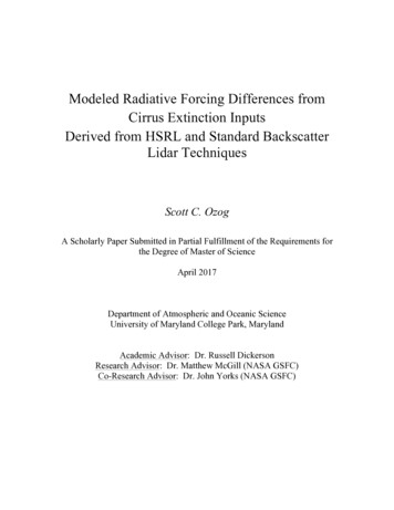
zero and is increased by intervals of 1.0 to a maximum of 100. The value that yields thebest reduced chi squared value when fit is determined to be the defect value for thatchannel.2.2 Improved Etalon CalibrationSince 2012 the ACATS instrument has flown in three field campaigns duringwhich etalon scans had been performed mid-flight. Etalon scans performed with zenithpointing lab data cannot be used on aircraft data because the environmental conditions atwhich the etalon operates are different. The temperature and pressure inside theinstrument are different in the lab than compared to flying on board the ER-2 at analtitude of 20km. Thus, etalon scans must be performed during in flight under theconditions that the etalon has been operating, and used to collect data. During these fieldcampaigns defect values retrieved from etalon calibration scans were not consistentlyreliable due to the non-uniformity of the signal from varying backscatter targets and thespeed of the aircraft (200 ms-1). Figures 4a and b show calibration fits from etalon scansperformed during ACATS’ last field campaign in August of 2015. The measured channelresponse is shown in red, and the fitted transmission function is shown in blue. Figure 4ais an example of the response in channel 1 from an etalon scan performed during a flighton August 19th, 2015. This response appears to have a good periodic structure and abroad fit transmission function. However, this example yielded defect values that weretoo high. Figure 4b shows the response in channel 13 from a flight the next day, and isan example of how poor the spectral response can be from in-flight calibration. To havethe most accurate etalon scan possible the signal must be invariant. It was originallydesigned that the stratospheric Rayleigh signal just below the aircraft would be used fora)b)Figure 4a. The calibration fit for ACATS channel 1 from an etalon scan performed on August 19th, 2015 with redrepresenting the spectral response, and blue the transmission function. (b) The calibration fit for channel 13 from ascan performed during a flight the next day on August 20th.calibration, but the molecular signal at this altitude was too weak for viable calibration.A new calibration technique has been successfully tested, and will soon beoperationally implemented, for improving the reliability of etalon scans that areperformed mid-flight. Instead of using the signal backscattered by the atmosphere, it wastheorized, and proven, that a scattering medium inside the ACATS telescope itself placed13

in the path of the laser could be used during calibration instead. This eliminates theaforementioned issue of a variable scene at high speeds resulting in inconsistent etalonscans. Etalon scans performed for zenith pointing ground data are also improved; as theyare susceptible to the same errors from a varying scene. A material that produces thepeak spectral response expected, and also withstands high intensity laser light on theorder of 30 minutes without experiencing any deformation was necessary. It wasdetermined that white Delrin plastic placed in the path of the laser achieved the desiredresults. However, using the delrin alone saturated the detectors so it was also discoveredthat neutral density filters along with a light dispersing element needed to be placed overthe fiber optic tip leading back into the optics box. Figure 5 shows the spectral responsein channel 1 from an etalon scan performed in the lab using this configuration. Theobserved sharp peak and near perfect fit of the transmission function is what’s expectedFigure 5. Spectral response in ACATS channel 1 from a etalon scan performed in the lab using thenew method of white delrin plastic inside the telescope as a scattering mediumin accurate etalon calibration.Once the optimal configuration was determined, testing began to ensure that thismethod was repeatable. To gain knowledge of the reliability of etalon scans from theprevious method, the etalon scans from the seven most recent field campaign flights werecompared to one another. Figure 6b is a plot showing the average defect values across allthe channels from those flights, as well as their standard deviation and coefficient ofvariation. The defect values recovered from the science flights are inconsistent andexhibit variability as high as almost 50% in some channels. For comparison seven etalonscans using the new method were run over the coarse of seven different days. Only onescan was done a day to mimic the conditions ACATS would operat

6 1. Introduction 1.1 Importance of Cirrus Cirrus clouds, which are composed of ice particles and found in Earth's upper troposphere, and sometimes lower stratosphere (Sassen, 1991; Murphy et al., 1990; Wang et al., 1996), play a crucial role in modulating Earth's radiative energy budget. Low and mid-level tropospheric clouds, composed of spherical liquid water droplets, are