WIXLIB

Texture AnalysisMichael A. Wirth, Ph.D.University of GuelphComputing and Information ScienceImage Processing Group 2004

What is Texture? Texture is a feature used to partition imagesinto regions of interest and to classify thoseregions. Texture provides information in the spatialarrangement of colours or intensities in animage. Texture is characterized by the spatialdistribution of intensity levels in aneighborhood.2

What is Texture? Texture is a repeating pattern of localvariations in image intensity:– Texture cannot be defined for a point.3

What is Texture? For example, an image has a 50% black and50% white distribution of pixels. Three different images with the sameintensity distribution, but with differenttextures.4

Texture Texture consists of texture primitives ortexture elements, sometimes called texels.– Texture can be described as fine, coarse, grained,smooth, etc.– Such features are found in the tone and structureof a texture.– Tone is based on pixel intensity properties in thetexel, whilst structure represents the spatialrelationship between texels.5

Texture– If texels are small and tonal differences betweentexels are large a fine texture results.– If texels are large and consist of several pixels, acoarse texture results.6

Texture Analysis There are two primary issues in textureanalysis:n texture classificationo texture segmentation Texture segmentation is concerned withautomatically determining the boundariesbetween various texture regions in an image. Reed, T.R. and J.M.H. Dubuf, CVGIP: Image Understanding, 57: pp.359-372. 1993.7

Texture Classification Texture classification is concerned withidentifying a given textured region from agiven set of texture classes.– Each of these regions has unique texturecharacteristics.– Statistical methods are extensively used.e.g. GLCM, contrast, entropy, homogeneity8

Defining Texture There are three approaches to definingexactly what texture is:c Structural: texture is a set of primitive texels insome regular or repeated relationship.d Statistical: texture is a quantitative measure of thearrangement of intensities in a region. This set ofmeasurements is called a feature vector.e Modelling: texture modelling techniques involveconstructing models to specify textures.9

Defining Texture Statistical methods are particularly usefulwhen the texture primitives are small,resulting in microtextures. When the size of the texture primitive is large,first determine the shape and properties ofthe basic primitive and the rules which governthe placement of these primitives, formingmacrotextures.10

Simple Analysis of Texture11

Range One of the simplest of the textureoperators is the range ordifference between maximum andminimum intensity values in aneighborhood.– The range operator converts theoriginal image to one in whichbrightness represents texture.12

Variance Another estimator of texture isthe variance in neighborhoodregions.– This is the sum of the squares ofthe differences between theintensity of the central pixel and itsneighbours.13

Quantitative Texture Measures Numeric quantities or statistics that describea texture can be calculated from theintensities (or colours) themselves14

Grey Level Co-occurrence The statistical measures described so far areeasy to calculate, but do not provide anyinformation about the repeating nature oftexture. A gray level co-occurrence matrix (GLCM)contains information about the positions ofpixels having similar gray level values.15

GLCM A co-occurrence matrix is a two-dimensionalarray, P, in which both the rows and thecolumns represent a set of possible imagevalues.– A GLCM Pd[i,j] is defined by first specifying adisplacement vector d (dx,dy) and counting allpairs of pixels separated by d having gray levels iand j.Pd [i , j ] nij– The GLCM is defined by:16

GLCM– where nij is the number of occurrences of the pixelvalues (i,j) lying at distance d in the image.– The co-occurrence matrix Pd has dimension n n,where n is the number of gray levels in the image.17

GLCM For example, if d (1,1)2 1 2 0 10 2 1 1 20 1 2 2 01 2 2 0 12 0 1 0 1ij0 2 20Pd 2 1 22 3 2101i22jthere are 16 pairs of pixels in the imagewhich satisfy this spatial separation. Sincethere are only three gray levels, P[i,j] is a 3 3matrix.18

GLCMAlgorithm: Count all pairs of pixels in which the first pixelhas a value i, and its matching pair displacedfrom the first pixel by d has a value of j. This count is entered in the ith row and jthcolumn of the matrix Pd[i,j] Note that Pd[i,j] is not symmetric, since thenumber of pairs of pixels having gray levels[i,j] does not necessarily equal the number ofpixel pairs having gray levels [j,i].19

Normalised GLCM The elements of Pd[i,j] can be normalised bydividing each entry by the total number ofpixel pairs.Normalised GLCM; N[i,j], defined by:P [i , j ]N [i , j ] P [i, j ]ijwhich normalises the co-occurrence values tolie between 0 and 1, and allows them to bethought of as probabilities.20

Numeric Features of GLCM Gray level co-occurrence matrices captureproperties of a texture but they are notdirectly useful for further analysis, such as thecomparison of two textures. Numeric features are computed from the cooccurrence matrix that can be used torepresent the texture more compactly.21

Maximum Probability This is simply the largest entry in the matrix,and corresponds to the strongest response.– This could be the maximum in any of the matricesor the maximum overall.Cm max Pd [i , j ]i, j22

Maximum Probability Maximum probability with w 21, and d (2,2)23

Moments The order k element difference moment canbe defined as:Momk (i j )k Pd [i , j ]ij This descriptor has small values in caseswhere the largest elements in P are along theprincipal diagonal. The opposite effect can beachieved using the inverse moment.Pd [i , j ]Momk ,i jkij (i j )24

Moments Moments with w 21, and d (2,2)25

Contrast Contrast is a measure of the local variationspresent in an image.C(k , n ) (i j ) Pd [i , j ]kinj– If there is a large amount of variation in an imagethe P[i,j]’s will be concentrated away from themain diagonal and contrast will be high.– (typically k 2, n 1)26

Contrast Contrast with w 21, and d (2,2)27

Homogeneity A homogeneous image will result in a cooccurrence matrix with a combination of highand low P[i,j]’s.Pd [i , j ]Ch ij 1 i j– Where the range of graylevels is small the P[i,j]will tend to be clustered around the main diagonal.– A heterogeneous image will result in an evenspread of P[i,j]’s.28

Homogeneity Homogeneity with w 21, and d (2,2)29

Entropy Entropy is a measure of information content.It measures the randomness of intensitydistribution.Ce Pd [i , j ]ln Pd [i , j ]ij– Such a matrix corresponds to an image in whichthere are no preferred graylevel pairs for thedistance vector d.– Entropy is highest when all entries in P[i,j] are ofsimilar magnitude, and small when the entries inP[i,j] are unequal.30

Entropy Entropy with w 21, and d (2,2)31

Correlation Correlation is a measure of image linearity [ijP [i, j ]] µ µdCc iijjσ iσ jµi iPd [i , j ], σ i2 i 2 Pd [i , j ] µi2 Correlation will be high if an image contains aconsiderable amount of linear structure.32

GLCM - References Carlson, G.E. and W.J. Ebel. "Co-occurrence matrix modification forsmall region texture measurement and comparison". in IGARSS'88Remote Sensing: Moving Towards the 21st Century, pp.519-520, IEEE,Edinburgh, Scotland. 1988.Argenti, F., L. Alparone, and G. Benelli, "Fast algorithms for textureanalysis using co-occurrence matrices". IEE Proceedings, Part F:Radar and SIgnal Processing, 137(6): pp. 443-448. 1990.Gotlieb, C.C. and H.E. Kreyszig, "textur descriptors based on cooccurrence matrices". Computer Vision, Graphics and ImageProcessing, 51(1): pp. 70-86. 1990.33

Problems with GLCM One problem with deriving texturemeasures from co-occurrence matricesis how to choose the displacementvector d.– The choice of the displacement vector is an important parameter in thedefinition of the GLCM.– Occasionally the GLCM is computed from several values of d and the onewhich maximises a statistical measure computed from P[i,j] is used.– Zucker and Terzopoulos used a χ2 measure to select the values of d thathave the most structure; i.e. to maximise2 the value:Pd [i , j ]χ (d ) 1ij Pd [ i ]Pd [ j ]234

Windowing Algorithms for texture analysis are applied toan image in a series of windows of size w,each centered on a pixel (i,j).– The value of the resulting statistical measure areassigned to the position (i,j) in the new pixel.35

Haralick Texture Operator Haralick et al. suggested a set of 14 texturalfeatures which can be extracted from the cooccurrence matrix, and which containinformation about image texturalcharacteristics such as homogeneity,linearity, and contrast. Haralick, R.M., K. Shanmugam, and I. Dinstein, "Textural features forimage classification". IEEE Transactions on Systems, Man andCybernetics: pp. 610-621. 1973.36

Graylevel Difference Statistics Grey-level differences are based on absoutedifferences between pairs of grey-levels. The grey-level differences are contained in a256-element vector, and are computed bytaking the absolute differences of all possiblepairs of grey levels distance d apart at angleθ, and counting the number of times thedifference is 0,1, ,25537

Graylevel Difference Statistics Let d (dx,dy) be the displacement vectorbetween two image pixels, and g(d) the graylevel difference at distance d.g (d ) f (i , j ) f (i dx, j dy ) pg(g,d) is the histogram of the gray-leveldifferences at the specific distance, d. Onedistinct histogram exists for each distance d.38

Graylevel Difference Statistics The difference statistics are then normalizedby dividing each element of the vector by thenumber of possible pixel pairs. Several texture measures can be extractedfrom the histogram of graylevel differences:39

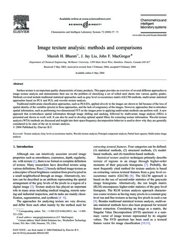
Graylevel Difference Statistics Mean:Nµd g k pg (g k , d )k 1– Small mean values µd indicate coarse texturehaving a grain size equal to or larger than themagnitude of the displacement vector. Entropy:NHd pg (g k , d )ln pg (g k , d )k 1– This is a measure of the homogeneity of thehistogram. It is maximised for uniform histograms.40

Graylevel Difference Statistics Variance:Nσ d2 (g k µd )2 pg (g k , d )k 1– The variance is a measure of the dispersion of thegray-level differences at a certain distance, d. Contrast:NCd g k2 pg (g k , d )k 141

Graylevel Difference StatisticsMeanStandard DeviationEntropyContrast42

Runlength Statistics The lengths of texture primitives in differentdirections can serve as a texture description.– A run length is a set of constant intensity pixelslocated in a line. Runlength statistics are calculated bycounting the number of runs of a given length(from 1 to n) for each grey level. Galloway, M.M., "Texture classification using gray level run lengths".Computer Graphics and Image Processing, 4(2): pp. 172-179. 1975.43

Runlength Statistics In a course texture it is expected that longruns will occur relatively often, whereas a finetexture will contain a higher proportion ofshort runs. Statistical measures:– Let B(a,r) be the number of primitives of alldirections having length r, and grey-level a, m andn the image dimensions, and L the LnumberofNrintensity values.K B(a, r )a 1 r 1– Let K be the number of runs:44

Runlength Statisticsc Long-run emphasis:Slr L1KNr2B(a,r)r a 1 r 1– This is a measure that emphasizes the long-runs of a graylevel image. Long-run emphasis will be large when there arelots of long runs of the same intensity.d Short-run emphasis: Ssr B(a, r ) 2ra 1 r 1L1KNr– This is a measure that emphasizes the short-runs of a graylevel image. short-run emphasis will be large whenthere are lots of short runs of the same intensity.45