WIXLIB

FEBRUARY 20212.2.Experiment designsWe conducted three historical simulation experimentsfor CAMS-CSM (Table 1). The first experiment “r1i1p1f1”starts from the initial conditions of 1 January 3025 of thepiControl experiment. The external forcing used for this simulation is from the recommendation of CMIP6 (https://esgfnode.llnl.gov/projects/input4mips), which includes historical GHG concentrations (CO2, CH4, N2O, CFC-12, and equivalent CFC-11, accounting for the radiative effects of all 39other gases) (Meinshausen et al., 2017), ozone concentrations -insupport-of-cmip6/), stratospheric aerosols (ftp://iacftp.ethz.ch/pub read/luo/CMIP6/data description.txt), and the totalsolar irradiance (http://solarisheppa.geomar.de/cmip6), aswell as the anthropogenic aerosols using simple plumes parameterization (Steven et al., 2016). Fixed land-use forcing isused in this simulation. The second simulation, “r2i1p1f1”,is the same as “r1i1p1f1” but starts from a different date ofpiControl (i.e., 1 January 3030). To identify the effect of volcanic eruptions, a third simulation, “r1i1p1f2 ”, is conducted, which is the same as “r1i1p1f1” but excludes the historical forcing of stratospheric aerosols. As required byCMIP6, all experiments were integrated from 1850 to 2014.3.287RONG ET AL.Data recordThe datasets of the CMIP6 historical experiments forCAMS-CSM have been published onto the ESGF dataserver and can be accessed via searching the model nametogether with the experiment name (i.e., “historical ”) athttps://esgf-data.dkrz.de/search/cmip6-dkrz/ or https://esgfnode.llnl.gov/projects/cmip6/. The data format is the Network Common Data Form (NetCDF), version 4, which canbe read and visualized by scientific data analysis and visualization software like the NCAR Command Language (NCL,http://www.ncl.ucar.edu) or Python (https:// www.python.org). Users can also process the data by command-linetoolkits such as the Climate Data Operator (CDO, https://code.mpimet.mpg.de/projects/cdo/) or the NetCDF Operator (NCO, http://nco.sourceforge.net).Monthly mean and daily mean outputs are provided forthe CAMS-CSM datasets. There are 38 monthly mean variables for the atmospheric model dataset, including air temperature, humidity, velocity, sea level pressure, precipitation,radiation fluxes, surface heat fluxes and momentum fluxes,cloud water and cloud ice, cloud cover, etc. In total, 11monthly mean variables of the oceanic model are provided,including sea temperature, salinity, velocity, surface heatflux, mixed-layer depth, sea surface height etc. The monthlymean outputs of the land model contain 10 variables, including soil temperature, soil moisture and ice, evaporation, etc.The sea-ice model provides 18 monthly mean variables,including sea-ice concentration, temperature, velocity, thickness, sea ice transport, surface stress, surface snow thickness, etc. The daily mean outputs are provided only for theatmospheric model, which contain 15 variables includingair temperature, velocity, humidity, surface temperature, precipitation, radiative fluxes, etc.4.ValidationThe datasets used in this study for validation consist ofthe surface air temperature of the Japanese 55-year Reanalysis (JRA-55) (Kobayashi and Iwasaki, 2016), land surface temperature data from the Climatic Research Unit Temperature, version 4 (CRUTEM4) (Osborn and Jones, 2014),sea-ice concentration from HadISST (Rayner et al., 2003),precipitation from the Global Precipitation ClimatologyProject (GPCP), version 2.3 (Adler et al., 2003), Levitus94ocean temperature data (Levitus and Boyer, 1994), and thecollaborative surface temperature data of HadCRUT4 of theMet Office Hadley Center and the Climatic Research Unitat the University of East Anglia (Morice et al., 2012). Thehorizontal grids of the JRA-55 data, GPCP data and HadCRUT4 data are 288 145, 144 72 and 72 36, respectively. The JRA-55 data and GPCP data are interpolated tothe CAMS-CSM grid for comparison.4.1.Climatology of temperature, precipitation and seaiceWe first examine two fundamental metrics for coupledclimate model performance: climatological annual mean surface air temperature and precipitation. Figure 1 shows the simulated and observed surface air temperature climatology. Itcan be seen that the model reproduces the global distribution of surface air temperature reasonably well. The overallspatial pattern of the simulated surface air temperatureresembles that from the observations. Over much of theocean and terrestrial areas, the biases are less than 1 C [globally averaged bias is 0.145 C, and the root-mean-squareerror (RMSE) is 2.42 C]. Evident biases primarily lie in theNorth Atlantic and the Southern Ocean near the Antarctic,where the biases can be larger than 5 C (with a significancelevel of 5%). The cold biases over the high latitudes of theTable 1. Experiment designs.Experiment id Variant labelIntegration timeExperiment designStarts from 1 January 3025 of the piControl experiment. The external forcing includeshistorical GHGs (CO2, CH4, N2O, CFC-12, and equivalent CFC-11), ozoneconcentrations, stratospheric aerosols, the total solar irradiance, andanthropogenic aerosols. Land-use forcing is fixed in this simulation.Same as r1i1p1f1, but starts from 1 January 3030 of the piControl experiment.Same as r1i1p1f1, but excludes the stratospheric aerosol toricalr2i1p1f1r1i1p1f21850–20141850–2014

288CAMS-CSM HISTORICAL SIMULATIONS DATASETSVOLUME 38Fig. 1. The climatology (1980–2014-averaged) of surface air temperature at 2m: (a) ensemble mean of CAMS-CSM historical simulations (r1i1p1f1 andr2i1p1f1); (b) JRA-55 data; (c) differences between CAMS-CSM historicalsimulations and JRA-55 data. The hatched areas in the plots denote thesignificance level of 5% from the t-test against the interannual anomalies.Units: C.North Atlantic are associated with the overestimated sea-icecover in the Northern Hemisphere, while the warm biasesnear the Antarctic might be ascribed to the underestimatedsea-ice extent over there. In the eastern coastal regions ofthe tropical Pacific and Atlantic, the simulated surface temperature tends to be warmer than observed, which is a usual feature of coupled climate models and may result from their inadequate representation of stratocumulus and coastalupwelling. We also calculated the surface air temperatureerror over land using CRUTEM4 data. The result showsthat the global mean biases and RMSE over land are 0.128 C and 2.14 C, respectively, which are smaller thanthose of the previous version ( 1.53 C and 2.31 C), suggest-ing a performance improvement in the CMIP6 version.Figure 2 shows the simulated and observed annualmean precipitation. Overall, the simulated precipitationshows a similar pattern to the observations (globally averaged bias of 0.03 mm d 1; RMSE of 1.15 mm d 1). The active precipitation centers, such as the intertropical convergence zone (ITCZ), South Pacific convergence zone(SPCZ), and South Atlantic convergence zone (SACZ), aswell as those over the tropical Indian Ocean and subtropical oceans, are reasonably captured by the model. Compared with the GPCP data, the simulated precipitation overthe tropical oceans is generally overestimated, especiallyover the areas of the ITCZ and SPCZ, where the biases can

FEBRUARY 2021RONG ET AL.289Fig. 2. The climatology (1980–2014-averaged) of precipitation: (a) ensemblemean of CAMS-CSM historical simulations (r1i1p1f1 and r2i1p1f1); (b)GPCP data; (c) differences between CAMS-CSM historical simulations andGPCP data. The hatched areas in the plots denote the significance level of 5%from the t-test against the interannual anomalies. Units: mm d 1.exceed 4 mm d 1 and the general precipitation pattern in thetropical Pacific tends to bear a double-ITCZ structure. Tosome extent, the double-ITCZ bias is improved comparedwith the previous version (Rong et al., 2018); however, itstill remains a prominent discrepancy of the CAMS-CSMmodel. Although it is recognized that the double-ITCZerrors arise from the Bjerknes feedback between atmosphere and ocean, how to eliminate this bias remains unresolved and the double-ITCZ still stands out as a prevailingerror in current coupled models (Zhang et al., 2015). Notably, the double-ITCZ bias has been largely reduced in theFGOALS-f3-L model (Guo et al., 2020), possibly benefiting from the convection scheme adopted in the model, andsuggesting that improving physical schemes might be aneffective way to eliminate the double-ITCZ error. Over thetropical Atlantic, the simulated SACZ shifts southward tothe warm SST bias area, with excessive precipitation in thetropical South Atlantic. Dry biases can be found in the central and eastern equatorial Pacific, as a result of an overestimated cold tongue in the model. A certain connection existsbetween the temperature biases and precipitation biasesover some land areas. For example, the warm biases over tropical Africa and the Amazon appear to be associated with thedryer biases over these regions, while the cold biases overthe Tibetan Plateau correspond to overestimated precipitation.The equatorial thermocline plays a crucial role in the climate variability of the tropical Pacific. Fluctuation of the ther-

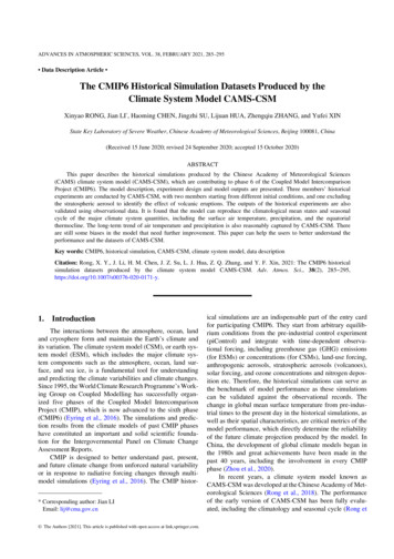
290CAMS-CSM HISTORICAL SIMULATIONS DATASETSmocline depth is tightly connected with the sea surface temperature anomalies associated with the ENSO phenomenon.Figure 3 shows the simulated annual mean upper-ocean temperature along the equatorial oceans. Here, we use the depthof the 20 C isotherm to represent the thermocline depth. Itcan be seen that the west–east-tilted feature of the equatorial Pacific thermocline is well depicted by the model. Inthe equatorial Pacific, the 20 C isotherm of the model generally follows that of the observation. The discrepancy is thatthe simulated thermocline exhibits a kind of weaker zonalslope compared with the observation, which is primarily manifested by a slightly shallower thermocline in the model inthe western Pacific. The 20 C isotherms in the IndianOcean and Atlantic Ocean are also reproduced reasonablywell, with a weaker slope relative to the observation. Below150 m in the Pacific Ocean, the isotherms generally followthe observation, while warm biases can be found over theIndian and Atlantic oceans.Figure 4 shows the climatological mean sea-ice concentration for the historical simulations. The line (thick cyan)of 15% mean concentration from the HadISST data is presented for comparison. In general, the model is able to depictthe seasonal evolution of sea-ice concentrations. During February–March–April, the simulated Arctic sea ice extendstoo much to the equator, in particular over the NorthAtlantic Ocean, whereas during August–September–October the sea-ice cover is in agreement with the observation.Analogous to the previous version (Rong et al., 2018), theAntarctic sea ice is underestimated by the model, especiallyduring February–March–April, and the sea ice is visibleover some areas of the Ross Sea and Weddell Sea. The excessive/insufficient sea-ice cover concentrations in the Arctic/Antarctic leads to the warm/cold biases in the surface temperature over these regions, indicating that the representation ofsea ice needs further improvement to enhance the temperature simulation.4.2.VOLUME 38Interannual variabilityFigures 5a and b show the standard deviation of theNiño3.4 index from the observations and model. It can beseen that the amplitude of the simulated Niño3.4 SST variability is closely consistent with the HadISST data. Similar tothe observation, the simulated ENSO tends to mature during the winter, indicating a reasonable phase-locking feature produced by the model. In particular, the overestimated ENSO amplitude in the previous version of CAMSCSM is remarkably reduced, which may be attributable tothe improvement in convection and cloud radiative forcingover the tropical Pacific due to the modification of the cumulus scheme. Note that in the current version there is a secondary peak occurring near May, which is not observed in the previous version. The spatial distribution of simulated SST variability also shows a reasonable pattern with respect to theobservation (Figs. 5a and b), with the maximum center situated over the central-eastern equatorial Pacific. Comparedwith the observation, the SST variance is underestimatedover the coastal region of South America, which is a common bias in coarse resolution coupled models and can beattributed to the insufficient coastal upwelling in these models.4.3.Long-term trendAs mentioned above, the change in global mean surface temperature from pre-industrial times to the presentday in the historical simulations is a key metric of the modelperformance. Figure 6a shows the simulated and observedglobal mean surface air temperature anomalies from 1850 to2014. It can be seen that all three ensemble members can reasonably capture the long-term warming trend since 1850, aswell as the rapid warming after 1980. As three ensemble members start from different initial conditions or using differentforcing, the transient phases among them are inconsistentexcept during the major volcanic eruption periods. ForFig. 3. Annual mean temperatures ( C) along the equator (5 S–5 N) derived from the CAMS-CSMhistorical simulation (black contours and shading) and Levitus94 climatology (white contours). Theblack and red thick lines indicate the 20 C isotherm from CAMS-CSM and the Levitus94climatology, respectively. units: C.

FEBRUARY 2021RONG ET AL.291Fig. 4. Climatological sea-ice concentration in the (a, b) Arctic and (c, d) Antarctic for the period 1980–2014 for thehistorical simulations. The thick cyan lines indicate the 15% mean concentration values from the HadISST data withthe same period. Panels (a, c) and (b, d) denote the averages for February–March–April and August–September–October, respectively. Units: %.example, the global mean surface air temperature of“r1i1p1f1” and “r2i1p1f1” shows notable decline near theeruption periods of Krakatoa (1883), Mount Pelée (1902)and Pinatubo (1991), while in “r1i1p1f2” such a global cooling is absent because the stratospheric aerosols are excludedin this simulation. Compared with the observations, the simulated cooling in responses to volcanic eruption is overestimated, especially during Pinatubo’s eruption, leading to aweaker warming in both the “r1i1p1f1” and “r2i1p1f1” experiments after the 1990s. The simulation of “r1i1p1f2 ”,however, shows a comparable warming trend to thatobserved. The averaged least-squares linear trends of thethree simulations from 1850 to 2014 are 0.041 (r1i1p1f1),0.040 (r2i1p1f1), and 0.046 (r1i1p1f2) C (10 yr) 1, whichis slightly weaker than that of the observation [0.048 C(10 yr) 1]. Note that the warming of “r1i1p1f2” after 1980is remarkably stronger than those of “r1i1p1f1 ” and“r2i1p1f1 ”. The linear trends of the HadCRUT4 data,“r1i1p1f1”, “r1i1p1f2” and “r1i1p1f2” from 1980 to 2014are 0.161, 0.137, 0.138 and 0.204 C (10 yr) 1, respectively,suggesting a robust cooling effect of Pinatubo in this model.It can be seen that the warming trend produced in CAMSCSM is weaker than that of the FGOALS-f3-L, in which thetrend tends to be greater than observed, suggesting different climate sensitivities of the two models. The observed precipitation time series exhibits a slight wetting trend after the1980s, which is captured by the three ensemble members’simulations. Before the 1980s, the simulated precipitationshows significant interannual fluctuation without an obvious long-term trend.Figure 7 shows the linear trend of the simulated andobserved zonal mean air temperature from 1960 to 2014. Ingeneral, the model captures well the major pattern of thetrend in air temperature from the surface to 10 hPa. The

292CAMS-CSM HISTORICAL SIMULATIONS DATASETSVOLUME 38Fig. 5. Standard deviation of the Niño3.4 index [SST anomaly averaged over (5 S–5 N, 170 –120 E)] for eachcalendar month as derived from the (a) HadISST data and (b) CAMS-CSM. Panels (c, d) show the standard deviationof SST anomalies from HadISST and CAMS-CSM, respectively. Units: C.observed trend of air temperature mainly shows a reversed distribution between the troposphere (below 150 hPa) and stratosphere (above 150 hPa), reflecting a typical structure of airtemperature changes in response to increasing GHGs(Fig. 7b). Over the polar region of the Southern Hemisphere, the observed trend exhibits a sandwich structure,i.e., a warming trend below 300 hPa and above 30 hPa, anda cooling trend between 300 hPa and 30 hPa. The model isable to reproduce the reversed trend between the troposphere and stratosphere, and the simulated magnitude of thetrend is comparable with that of the observation. Noting thatthe complex structure over the southern polar region is successfully captured by the model, especially the warming center above 30 hPa, which seems absent in FGOALS-f3-L(Guo et al., 2020), there are nonetheless some deficienciesin the model. For example, the maximum cooling in themodel shifts toward to the lower stratosphere, and the warming trend in the lower troposphere over the southern and northern polar regions is somewhat underestimated.5.Usage notesAs the top of the atmospheric model is 10 hPa, the values above 10 hPa are unrealistic and have been filled withmissing values in the atmospheric pressure level datasets.The ocean component (MOM4) and sea-ice component (SIS) of CAMS-CSM use a tripolar grid, which is composed of a bipolar Arctic grid (two northern poles areplaced over the North American and Eurasian land areas)and a normal spherical latitude–longitude grid. As the tripolar grid model uses generalized orthogonal curvilinearcoordinates, its X and Y directions are orthogonal over thebipolar region, but no longer parallel to latitude–longitudecircles. Instead, there are geographically varying anglesbetween two grids. At present, the oceanic and sea-ice output dataset of CAMS-CSM published on the ESGF node areon the original tripolar grid (i.e., the grid label “gn” meansthe model’s native grid), and thus specific consideration isrequired before visualization of the datasets. For scalar variables, users can directly analyze and visualize the dataset bysoftware that supports curvilinear grids (i.e., the grids represented by two-dimensional latitude/longitude arrays), such asNCL or Python. An alternative choice is to interpolate the original data to a latitude–longitude grid using CDO or NCO,which can be easily processed by command-line operations.For vector variables over the latitude–longitude grid area(southward of 60 N), users can directly analyze or visualize the data using normal scientific data analysis and visualiza-

FEBRUARY 2021RONG ET AL.293Fig. 6. Global mean (a) surface air temperature (unit: C) and (b) precipitation (units: mm d 1) anomalies(annual mean) relative to the period 1961–90 for the CAMS-CSM historical experiments and observation.The observational data for surface air temperature and precipitation are HadCRUT4 and GPCP, respectively.Fig. 7. Linear trends of zonal mean air temperature from 1960 to 2014 for the (a) ensemble mean of the CAMS-CSMhistorical experiments (r1i1p1f1 and r2i1p1f1) and (b) observation (JRA-55).tion software. While over the bipolar Arctic region poleward of 60 N, rotations are needed before visualization

ation, a couple of updates have been made for CAMS-CSM to improve its simulation of cloud radiative forcing and radi-ation transfer. This new version of CAMS-CSM is the one that is running the formal CMIP6 simulations. At the time of writing, CAMS-CSM has completed all the entry card sim-ulations of CMIP6, and the model outputs have been pub-