Transcription
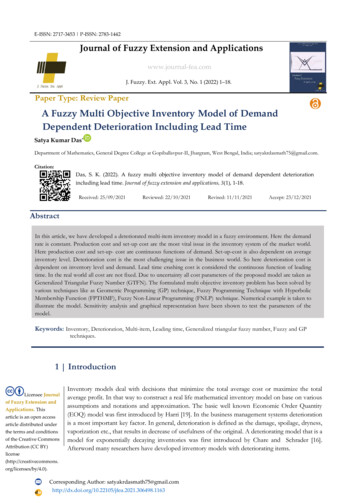
E-ISSN: 2717-3453 P-ISSN: 2783-1442Journal of Fuzzy Extension and Applicationswww.journal-fea.comJ. Fuzzy. Ext. Appl. Vol. 3, No. 1 (2022) 1–18.Paper Type: Review PaperA Fuzzy Multi Objective Inventory Model of DemandDependent Deterioration Including Lead TimeSatya Kumar Das*Department of Mathematics, General Degree College at Gopiballavpur-II, Jhargram, West Bengal, India; satyakrdasmath75@gmail.com.Citation:Das, S. K. (2022). A fuzzy multi objective inventory model of demand dependent deteriorationincluding lead time. Journal of fuzzy extension and applications, 3(1), 1-18.Received: 25/09/2021Reviewed: 22/10/2021Revised: 11/11/2021Accept: 23/12/2021AbstractIn this article, we have developed a deteriorated multi-item inventory model in a fuzzy environment. Here the demandrate is constant. Production cost and set-up cost are the most vital issue in the inventory system of the market world.Here production cost and set-up- cost are continuous functions of demand. Set-up-cost is also dependent on averageinventory level. Deterioration cost is the most challenging issue in the business world. So here deterioration cost isdependent on inventory level and demand. Lead time crashing cost is considered the continuous function of leadingtime. In the real world all cost are not fixed. Due to uncertainty all cost parameters of the proposed model are taken asGeneralized Triangular Fuzzy Number (GTFN). The formulated multi objective inventory problem has been solved byvarious techniques like as Geometric Programming (GP) technique, Fuzzy Programming Technique with HyperbolicMembership Function (FPTHMF), Fuzzy Non-Linear Programming (FNLP) technique. Numerical example is taken toillustrate the model. Sensitivity analysis and graphical representation have been shown to test the parameters of themodel.Keywords: Inventory, Deterioration, Multi-item, Leading time, Generalized triangular fuzzy number, Fuzzy and GPtechniques.1 IntroductionLicensee Journalof Fuzzy Extension andApplications. Thisarticle is an open accessarticle distributed underthe terms and conditionsof the Creative CommonsAttribution (CC BY)Inventory models deal with decisions that minimize the total average cost or maximize the totalaverage profit. In that way to construct a real life mathematical inventory model on base on variousassumptions and notations and approximation. The basic well known Economic Order Quantity(EOQ) model was first introduced by Harri [19]. In the business management systems deteriorationis a most important key factor. In general, deterioration is defined as the damage, spoilage, dryness,vaporization etc., that results in decrease of usefulness of the original. A deteriorating model that is amodel for exponentially decaying inventories was first introduced by Chare and Schrader [16].Afterword many researchers have developed inventory models with deteriorating by/4.0).Corresponding Author: .doi.org/10.22105/jfea.2021.306498.1163
In the real situation of the business world many inventory control model involves the deterministic leadtimes. Ben-Daya and Raouf [4] studied an inventory model involve the lead-time as a decision variable.Hariga and Ben-Daya [18] developed some stochastic inventory model with deterministic variable leadtime. Chuang et al. [9] presented a note on periodic review inventory model with controllable setup costand lead time. Ouyang [24] considered a mixture inventory model with backorders and lost sales forvariable lead time also in [25] developed a min-max distribution free procedure for mixed inventorymodel with variable lead time. Sarkar et al. [29] established an integrated inventory model with variablelead time, defective units and delay in payments. Sarkar et al. [30] discussed a quality improvement andbackorder price discount under controllable lead time in an inventory model. Multi items are used tofulfill customers demands as well as to increase the maximum profit of business men. Kotb and Fergany[22] developed a multi-item EOQ model with both demand dependet unit cost and varying lead time.Abou-El-Ata and Kotb [1] used a multi-item EOQ inventory model with varying holding cost undertwo restrictions. Saha and Sen [36] published a paper on inventory model with negative exponentialdemand and probabilistic deterioration under backlogging. Das and Islam [15] considered multiobjective two echelon supply chain inventory model with customer demand dependent purchase costand production rate dependent production cost. Das [37] developed multi item inventory model includelead time with demand dependent production cost and set-up-cost in fuzzy environment.The concept of fuzzy set theory was first introduced by Zadeh [34]. Afterward Zimmermann [35]applied the fuzzy set theory concept with some useful membership functions to solve the linearprogramming problem with some objective functions. Bit [3] studied fuzzy programming withhyperbolic membership functions for multi objective capacitated transportation problem. Maiti [23]considered fuzzy inventory model with two warehouse under possibility measure in fuzzy goal. AlsoGeometric Programming (GP) is a powerful optimization technique developed to solve a class of nonlinear optimization programming problems especially found in engineering design and manufacturing.Multi objective GP techniques are also interesting in the EOQ model. GP was introduced by Duffin etal. [12]. Beightler and Phillips [5] applied GP. Biswal [6] considered fuzzy programming technique tosolve multi- objective GP problems. Das et al. [14] established a multi-item inventory model withquantity dependent inventory costs and demand-dependent unit cost under imprecise objective andrestrictions in GP approach. Mandal et al. [27] presented a multi-objective fuzzy inventory model withthree constraints in a GP approach also used this method in [28] developed an inventory model ofdeteriorating items with a constraint. Islam [21] solved multi-objective marketing planning inventorymodel. Islam [20] discussed multi-objective geometric-programming problem and its application.Barman et al. [39] developed an analysis of retailer’s inventory in a two-echelon centralized supply chainco-ordination under price-sensitive demand.2Das J. Fuzzy. Ext. Appl. 3(1) (2022) 1-18Aggarwal [2] studied a note on an order-level inventory model for a system with constant rate ofdeterioration. Dave and Patel [10] developed (T. Si) policy inventory for deteriorating items with timeproportional demand. Dave [11] developed a order level inventory model for deteriorating items withvariable instantaneous demand and discrete opportunities for replacement. Chen [8] studied an optimaldetermination of quality level, selling quantity and purchasing price for intermediate firms. Goyal andGiri [17] presented recent trends in modeling of deteriorating inventory. Wee et al. [33] considered amulti-objective joint replenishment inventory model of deteriorated items in a fuzzy environment.Tripathi et al. [32] discussed an inventory model with exponential time-dependent demand rate, variabledeterioration, shortages and production cost. Shaikh et al. [31] established a fuzzy inventory model fora deteriorating item with variable demand, permissible delay in payments and partial backlogging withShortage Follows Inventory (SFI) policy. Das and Islamn [13] proposed two warehouse inventory modelfor deteriorating items and Stock dependent demand under conditionally permissible delay in payment.Chakraborty et al. [7] derived two-warehouse partial backlogging inventory model with ramp typedemand rate, three-parameter Weibull distribution deterioration under inflation and permissible delayin payments. Panda et al. [26] explored a credit policy approach in a two-warehouse inventory modelfor deteriorating items with price-and stock-dependent demand under partial backlogging.
3In this paper, we have developed a deteriorated multi-item inventory model in a fuzzy environment. HereProduction cost, set-up- cost and deterioration cost are continuous functions of constant demand. Set-upcost and deterioration costs are also dependent on average inventory level. Lead time crashing cost isconsidered the continuous function of leading time. Due to uncertainty all cost parameters of the proposedmodel are taken as Generalized Triangular Fuzzy Number (GTFN). The formulated multi objectiveinventory problem has been solved by various techniques like as GP, FPTHMF, and FNLP. Numericalexample is taken to illustrate the model. Sensitivity analysis and graphical representation have been shownto test the feasibility of the model for various parameters of the model. Finally conclusions have beendrowning.2 Mathematical Model2.1 NotationsA fuzzy multi objective inventory model of demand dependent deterioration including lead timeℎ𝑖 : Holding cost per unit per unit time for ith item.𝑇𝑖 : The length of cycle time for 𝑖thitem, 𝑇𝑖 0.𝐷𝑖 : Demand rate per unit time for the ith item.𝐿𝑖 : Length of leading time for the ith item.𝑆𝑆𝑖 : Safety stock for the ith item.𝐼𝑖 (𝑡): Inventory level of the ith item at time t.𝑄𝑖 : The order quantity for the duration of a cycle of length 𝑇𝑖 for ith item.𝑇𝐴𝐶𝑖 (𝐷𝑖 , 𝑄𝑖 , 𝐿𝑖 ): Total average profit per unit for the ith item.𝑤𝑖 : Storage space per unit time for the ith item.𝑊 : Total area of space.𝑘: Safety factor.𝜃𝑖 : Constant deterioration rate for the ith item.̃𝑖 : Fuzzy storage space per unit time for the ith item.𝑤ℎ̃𝑖 : Fuzzy holding cost per unit per unit time for the ith item.̃𝑖 (𝐷𝑖 , 𝑄𝑖 , 𝐿𝑖 ): Fuzzy total average cost per unit for the ith item.𝑇𝐴𝐶̂𝑖 : Defuzzyfication of the fuzzy number 𝑤̃𝑖 .𝑤ℎ̂𝑖 : Defuzzyfication of the fuzzy number ℎ̃𝑖 .̂𝑖 (𝐷𝑖 , 𝑄𝑖 , 𝐿𝑖 ): Defuzzyfication of the fuzzy number 𝑇𝐴𝐶̃𝑖 (𝐷𝑖 , 𝑄𝑖 , 𝐿𝑖 ).𝑇𝐴𝐶
2.2 AssumptionsI.II.III.IV.V.Multi-item is considered.The replenishment rate is instantaneously and infinite.The lead time is allowed.Shortage is not considered.The unit production cost 𝐶𝑖𝑝 of ith item is inversely related to the demand rate 𝐷𝑖 . So we take theVI.following form 𝐶𝑖𝑝 ( 𝐷𝑖 ) 𝛼𝑖 𝐷𝑖 𝛽𝑖 , where 𝛼𝑖 0, 𝛽𝑖 1 are real constant.The set up cost is related to the average inventory level as well as demand. So we take the form𝑄 𝛿𝑖4𝜎𝑆𝑐 𝑖 (𝑄𝑖 , 𝐷𝑖 ) 𝛾𝑖 ( 2𝑖 ) 𝐷𝑖 𝑖 where 0 𝛾𝑖, 0 𝛿𝑖 1 & 0 𝜎𝑖 1 are real constant.Lead time crashing cost is related to the lead time by a function of the form 𝑅𝑖 ( 𝐿𝑖 ) 𝜌𝑖 𝐿𝑖 𝜏𝑖 , where𝜌𝑖 0 and 0 𝜏𝑖 0.5 are real constant.VII.𝑆𝑆𝑖 𝑘𝜔 𝐿𝑖.VIII.Q i ϕi φiθc (Q) υi ( ) D i .2IX.iform where0 𝜐𝑖 1, 𝜑𝑖 1 and 0 𝜙𝑖 1 are constant real numbers.2.3 Formulation of the ModelThe inventory situation for ith item is illustrated in Fig. 1. During the period the inventory level decreasesdue to demand rate and the deterioration rate. In the time interval [0, 𝑇𝑖 ] the satisfying differentialequation isdIi (t)dt θi I i (t) D i,0 t Ti .(1)With boundary conditions, 𝐼𝑖 (0) 𝑄𝑖 , 𝐼𝑖 (𝑇𝑖 ) 0.Solves the Eq (1) using the boundary conditions we have,DDiiI i (t) e θi t ( θ i Q i ) θ i , 0 t Ti ,(2) Q i (D i Q i θi )t (Neglected square and higher power of θi since θi 1).Ti Qi.(D i Q i θi )(3)Now various average costs for ith item areI. Average production cost (𝑃𝐶𝑖 ) 𝑄𝑖 𝐶𝑖𝑝 ( 𝐷𝑖 )𝑇𝑖 𝛼𝑖 (𝐷𝑖 (1 𝛽𝑖) 𝑄𝑖 𝜃𝑖 𝐷𝑖 𝛽𝑖 ).𝑇1𝑄II. Average inventory holding cost (𝐻𝐶𝑖 ) 𝑇 𝑖 ℎ𝑖 𝐼𝑖 (𝑡)𝑑𝑡 ℎ𝑖 𝑘𝜔 𝐿𝑖 ℎ𝑖 ( 2𝑖 𝑘𝜔 𝐿𝑖 ).𝑖 0III. Average set-up-cost (𝑆𝐶𝑖 ) Das J. Fuzzy. Ext. Appl. 3(1) (2022) 1-18The deterioration cost is proporsonaly related to the average inventory level. So we take the1𝑇𝑖𝑄𝑖 𝛿𝑖𝜎 1𝜎[𝛾𝑖 ( 2 ) 𝐷𝑖 𝑖 ] IV. Average lead time crashing cost (𝐶𝐶𝑖 ) 𝜌𝑖 𝐿𝑖 𝜏𝑖𝑇𝑖𝛾𝑖 𝑄𝑖 𝛿𝑖 1 (𝐷𝑖 𝑖 𝑄𝑖 𝜃𝑖 𝐷𝑖 𝜎𝑖 )2𝛿 𝑖𝜌𝑖 𝐿𝑖 𝜏𝑖 (𝐷𝑖 𝑄𝑖 𝜃𝑖 )𝑄𝑖.
𝑄 𝜙𝑖V. Average deterioration cost (𝐷𝐶𝑖 ) 𝜃𝑖 𝜐𝑖 ( 2𝑖 ) 𝐷𝑖 𝜑𝑖 .Total average cost per unit time for ith item is5TAC i (D i , Q i , L i ) (PC i HC i SC i CC i DC i ) αi (D i (1 βi ) Q i θi D i βi ) σ 1QiA fuzzy multi objective inventory model of demand dependent deterioration including lead timeh i ( 2 kω L i ) γi Qi δi 1 (Di i Qi θi Di σi )2δi ρi Li τi (Di Qi θi )QiQi ϕi θi υi ( 2 ) D i φi(4).Inventory LevelFig. 1. For the ith item.So our Multi-Objective Inventory Model (MOIM) is defined as:Min {TAC 1 , TAC 2 , TAC 3 , , TAC n },QTAC i (D i , Q i , L i ) αi (D i (1 βi ) Q i θi D i βi ) h i ( 2i kω L i ) σ 1γi Qi δi 1 (Di i Qi θi Di σi )2δi ρi Li τi (Di Qi θi ) QiQ ϕiθi υi ( 2i ) D i φi ,Subject to, D i 0, Q i 0, L i 0, for i 1,2, . . n.2.4 Fuzzy ModelFor uncertainty, all the cost parameters of the model are taken as GTFN. The GTFN are assume as𝛼̃𝑖 (𝛼𝑖 1 , 𝛼𝑖 2 , 𝛼𝑖 3 ; 𝜓𝛼𝑖 ), 0 𝜓𝛼𝑖 1; ℎ̃𝑖 (ℎ𝑖 , ℎ𝑖 , ℎ𝑖 ; 𝜓ℎ𝑖 ), 0 𝜓ℎ𝑖 1,123𝛽̃𝑖 (𝛽𝑖 1 , 𝛽𝑖 2 , 𝛽𝑖 3 ; 𝜑𝛽𝑖 ), 0 𝜑𝛽𝑖 1; 𝜌̃𝑖 (𝜌𝑖 1 , 𝜌𝑖 1 , 𝜌𝑖 1 ; 𝜓𝜌𝑖 ), 0 𝜓𝜌𝑖 1,̃𝑖 (𝜃𝑖 1 , 𝜃𝑖 2 , 𝜃𝑖 3 ; 𝜓𝜃 ), 0 𝜓𝜃 1; 𝜏̃𝑖 (𝜏𝑖 1 , 𝜏𝑖 2 , 𝜏𝑖 3 ; 𝜓𝜏 ), 0 𝜓𝜏 1,𝜃𝑖𝑖𝑖𝑖𝛾̃𝑖 (𝛾𝑖 1 , 𝛾𝑖 2 , 𝛾𝑖 3 ; 𝜓𝛾𝑖 ), 0 𝜓𝛾𝑖 1; 𝜐̃𝑖 (𝜐𝑖 1 , 𝜐𝑖 2 , 𝜐𝑖 3 ; 𝜓𝜐𝑖 ), 0 𝜓𝜐𝑖 1,𝛿̃𝑖 (𝛿𝑖 1 , 𝛿𝑖 2 , 𝛿𝑖 3 ; 𝜓𝛿𝑖 ), 0 𝜓𝛿𝑖 1; 𝜎̃𝑖 (𝜎𝑖 1 , 𝜎𝑖 2 , 𝜎𝑖 3 ; 𝜓𝜎𝑖 ), 0 𝜓𝜎𝑖 1,(5)
̃𝑖 (𝜙𝑖 1 , 𝜙𝑖 2 , 𝜙𝑖 3 ; 𝜓𝜙 ), 0 𝜓𝜙 1; 𝜑̃𝑖 (𝜑𝑖 1 , 𝜑𝑖 2 , 𝜑𝑖 3 ; 𝜓𝜑𝑖 ), 0 𝜓𝜑𝑖 1,𝜙𝑖𝑖For 𝑖 1,2, , 𝑛.So our inventory Model (5) becomes the fuzzy model as6̃1 , TAC̃2 , TAC̃3 , . , TAC̃n },{TACMinSubject to, D i 0, Q i 0, L i 0, for i 1,2, . . n.̃̃i D i βi ) h̃i (Qi kω L i ) ̃i (D i (1 βi) Q i θTAC ̃i (D i , Q i , L i ) α2̃σ̃ 1δi 1(Di iγ̃Qi ĩi Di σ̃i ) Qi θ̃2δi τ̃ĩi )(Di Qi θρ̃Li iQi(6)̃ϕQ ĩi υ θ̃i ( i) D i φ̃i .2It is positioned that ranking fuzzy number is very important in the fuzzy programming system. Bortolanand Degani [38] established a number of techniques of ranking fuzzy numbers. 𝜆- integer method is usedfor defuzzification of fuzzy numbers. We know that approximated value of a GTFN 𝐴̃ (𝑎, 𝑏, 𝑐; 𝜓) is𝑎 2𝑏 𝑐given by 𝜓 (4) when 𝜆 0.5.Therefore the fuzzy inventory Model (6) converted tô1 , TAĈ2 , TAĈ3 , . , TAĈn },Min {TACSubject to, D i 0, Q i 0, L i 0,̂̂Q̃i D i βi ) ĥi ( i kω L i ) ̂i (D i (1 βi ) Q i θWhere TAĈi (D i , Q i , L i ) α2̂σ̂ 1γ̂i Qi δi 1 (Di ĩi Di σ̂i ) Qi θ̃̂2δi ̃i )ρ̂i Li τ̂i (Di Qi θQîϕ̂i υ̂i (Qi ) i D i φ̂i θ2(7)for i 1,2, . . n.3 Fuzzy Programming Techniques to Solve MOIMSolve the MOIM (7) as a single objective NLP using only one objective at a time and we ignoring theothers. So we get the ideal solutions. Using the ideal solutions we have got prepared the pay-off matrixas follows:TAC 1 (D 1 , Q 1 , L 1 )(D 11 , Q 11 , L11 )(D 22 , Q 22 , L22 )TAC 1 (D 11 , Q 11 , L11 )TAC 2 (D 11 , Q 11 , L11 ) .TAC n (D 11 , Q 11 , L11 )TAC 1 (D 22 , Q 22 , L22 )TAC 2 (D 22 , Q 22 , L22 ) TAC n (D 22 , Q 22 , L22 ) (D nn , Q nn , Lnn )TAC 2 (D 2 , Q 2 , L 2 ) . . .TAC n (D n , Q n , L n ) . . . .TAC 1 (D nn , Q nn , Lnn ) . . . .(8) . .TAC 2 (D nn , Q nn , Lnn ) TAC n (D nn , Q nn , Lnn )Let 𝑈 𝑘 𝑚𝑎𝑥 {𝑇𝐴𝐶𝑘 (𝐷𝑖𝑖 , 𝑄𝑖𝑖 , 𝐿𝑖𝑖 ), 𝑖 1,2, . , 𝑛} 𝑓𝑜𝑟 𝑘 1,2, . , 𝑛 and 𝐿𝑘 𝑇𝐴𝐶𝑘 (𝐷𝑘𝑘 , 𝑄𝑘𝑘 , 𝐿𝑘𝑘 )𝑓𝑜𝑟 𝑘 1,2, . , 𝑛.Das J. Fuzzy. Ext. Appl. 3(1) (2022) 1-18Where
Hence 𝑈 𝑘 , 𝐿𝑘 are identified, 𝐿𝑘 𝑇𝐴𝑃𝑘 (𝐷𝑖𝑖 , 𝑄𝑖𝑖 , 𝐿𝑖𝑖 ) 𝑈 𝑘 , 𝑓𝑜𝑟 𝑖 1,2, . , 𝑛 ; 𝑘 1,2, . , 𝑛.3.1 Fuzzy Programming Technique Using Hyperbolic Membership Function(FPTHMF)7Now fuzzy non-linear hyperbolic membership functions 𝜇𝐻𝑇𝐴𝐶𝑘 (𝑇𝐴𝐶𝑘 (𝐷𝑘 , 𝑄𝑘 , 𝐿𝑘 )) for the kth objectivefunction 𝑇𝐴𝐶𝑘 (𝐷𝑘 , 𝑄𝑘 , 𝐿𝑘 ) respectively for 𝑘 1.2. , . 𝑛 are defined as follows:1U k Lk1(TAC(D))(D)μH,Q,L tanh TAC,Q,Lσ kkkkkkkkkTACk) ) 2.(( 22Where 𝛼𝑘 is a parameter, 𝜎𝑘 3(𝑈 𝑘 𝐿𝑘 ) 2 6𝑈 𝑘 𝐿𝑘.A fuzzy multi objective inventory model of demand dependent deterioration including lead timeUsing the above membership function, fuzzy non-linear programming problem is formulated as follows:Max λSubject to12tanh ((Uk Lk21 TAC k (D k , Q k , L k )) σk ) 2 λ , λ 0.After simplification the above non-linear programming problem can be written asMax ySubject to y σk TAC k (D k , Q k , L k ) Uk Lk2σk , y 0, D k , Q k 0, L k 0.Now the above problem can be easily solved by suitable mathematical programming algorithm and thenwe shall get the solution of the MOIM (7).3.2 Fuzzy Non-Linear Programming Technique (FNLP) Based on Max-MinOperatorIn this technique fuzzy membership function 𝜇𝑇𝐴𝐶𝑘 (𝑇𝐴𝐶𝑘 (𝑄𝑘 . 𝐷𝑘 ))𝑇𝐴𝐶𝑘 (𝐷𝑘 , 𝑄𝑘 , 𝐿𝑘 ) respectively for 𝑘 1.2. , . 𝑛 are defined as follows:for the kth objective functionμTACk (TAC k (D k , Q k , L k ))1for TAC k (D k , Q k , L k ) LkU k TAC k (D k , Q k , L k ) for Lk TAC k (D k , Q k , L k ) U k ,U k Lk{0for TAC k (D k , Q k , L k ) U kfor k 1.2. , . n,Using the above membership function, fuzzy non-linear programming problem is formulated asMax α′subject to TAC k (D k , Q k , L k ) α′ (U k Lk ) U k .0 α′ 1, D k , Q k 0, L k 0.for k 1.2. , . n.
Now the above problem can be easily solved by suitable mathematical programming algorithm and thenwe shall get the solution of the MOIM (7).4 Geometric Programming TechniqueLet us consider a unconstrainted Multi Objective Geometric Programming (MOGP) problem is asfollows8T skj0Minimize g s (t) k 1c sk m, s 1.2.3. , , . n.j 1 t jSubject to t j 0. j 1.2. . m,Where 𝑐𝑠𝑘 ( 0) and 𝑠𝑘𝑗 (𝑗 1,2, . , 𝑚; 𝑘 1,2, . . . 𝑇0 ; 𝑠 1,2,3, . . , 𝑛) are all real numbers. Nowintroducing the weights 𝑤𝑖 (𝑖 1,2,3, . . , 𝑛), the above MOGP converted into the single objectiveGP problem as followingMinimize g(t) ns 1 w s g s (t), s 1.2.3. , , . n,T skj0i.e ns 1 k 1w s c sk m,j 1 t j(9)Subject to t j 0. j 1.2. . m.n i 1w i 1. w i 0. i 1.2.3. , , . n,Let 𝑇 be the total numbers of terms and 𝑚 is the number of variables. Then the degree of the difficulty(DD) is 𝑇 (𝑚 1).Dual Program: The dual problem of Eq. (9) is given as follows:To(Maximize v(θ) ns 1 k 1ws cskθskθsk).Subject toT0 ns 1 k 1θsk 1.(Normality condition)Ts0 ns 1 k 1 skj θsk 0.(Orthogonality conditions)θsk 0.(Positivity conditions)( j 1.2. , . m; k 1.2. , , , To ; s 1.2.3. , , . n).Now here three cases may arisesCase I: 𝑇0 𝑚 1, (i.e. DD 0). So DP presents a system of linear equations for the dual variables. Sowe have a unique solution vector of dual variable.Case II: 𝑇0 𝑚 1, So a system of linear equations is presented for the dual variables, where thenumber of linear equations is less than the number of dual variables. So it is concluded that dual variablevector has many solutions.Case III: 𝑇0 𝑚 1, so a system of linear equations is presented for the dual variables, where thenumber of linear equations is greater than the number of dual variables. It is seen that generally nosolution vector exists for the dual variables here.Das J. Fuzzy. Ext. Appl. 3(1) (2022) 1-18Primal Problem:
4.1 Solution Procedure of My Proposed ProblemPrimal Problem:9Minimize TAC(D. Q. L) ni 1 w i (α̂i (D îσ̂ 1γ̂i Qi δi 1 (Di ĩi Di σ̂i ) Qi θ ̃̂2δĩi )ρ̂i Li τ̂i (Di Qi θQi(1 β̂i )̃i D i β̂i ) ĥi (Qi kω L i ) Q iθ2̂iϕ̂i υ̂i (Qi ) D i φ̂i ), θ2(10)Subject to, D i 0, Q i 0, L i 0,n i 1w i 1. w i 0. i 1.2.3. , , . n,Dual Program: The dual problem of the primal problem Eq. (10) is as follows:A fuzzy multi objective inventory model of demand dependent deterioration including lead timeMaximize v(θ)nθi1w i α̂i ()θi1i 1̃w i ρ̂θi i()θi8θi8(θi2̃i α̂iwiθ()θi2̂i υ̂iw iθ̂2ϕi θi9w i ĥi()2θi3θi3θi4w i kωĥi()θi4(w i γ̂i2δ̂i θi5θi5)(̃w i γ̂θi i2δ̂i θi6θi6)θi7w i ρ̂i()θi7θi9) .Subject to θi1 θi2 θi3 θi4 θi5 θi6 θi7 θi8 θi9 1.(11)(1 β̂i )θi1 β̂i θi2 (σ̂i 1)θi5 σ̂θ̂i θi9 0.i i6 θi7 φ̂i θi9 0.θi2 θi3 (δ̂i 1)θi5 δ̂i θi6 θi7 ϕθi4 τ̂(θi i7 θi8 ) 2n i 1w i 1. w i 0.0.θi1 . θi2 . θi3 . θi4 . θi5 . θi6 . θi7 . θi8 . θi9 0 for i 1.2.3. , , . n.Solving the above linear equations we havêi (σ̂i 1) φ̂i σ̂i δ̂i φ̂i )θi7̂i θi3 {ϕ̂i (δ̂i 1)}θi5 (ϕ̂i )θi6 (φ̂i ϕθi2 [ φ(12)̂i θi1 ], (1 β̂i )ϕθi4 2τ̂θi i7 ̂i β̂i )(β̂i ϕ2(1 β̂i )2τ̂i1 θ1 θi3i1[{̂i φ̂i φ(1 2τ̂)(β̂i ϕ̂i )} (β̂i ϕ̂i )i ̂i (σ̂i 1) φ̂i φ̂i (δ̂i 1) β̂i ϕ̂i β̂i (δ̂i 1) (σ̂i 1)ϕ̂i φ(β̂i ϕ̂i )(13)̂i δ̂i φ̂i φ̂i δ̂i β̂i ϕ̂i β̂i δ̂i σ̂iϕ θi6̂i φ(β̂i ϕ̂i ) ̂i β̂i ϕ̂i 1 β̂i 2τ̂(β̂ ̂ ̂i )̂i ϕ2φi i ϕi φ̂i φ(β̂i ϕ̂i )θi5θi7 ],
θi8 ̂i β̂i )(β̂i ϕ2(1 β̂i )11 θ1 θi3i1 {[̂i φ̂i φ(1 2τ̂)(β̂i ϕ̂i )} (β̂i ϕ̂i )i ̂i (σ̂i 1) φ̂i φ̂i (δ̂i 1) β̂i ϕ̂i β̂i (δ̂i 1) (σ̂i 1)ϕ̂i φ(β̂i ϕ̂i )θi5(14)̂i δ̂i φ̂i φ̂i δ̂i β̂i ϕ̂i β̂i δ̂i σ̂iϕ θi6̂i φ(β̂i ϕ̂i ) θi9 1̂i φ(β̂i ϕ̂i )̂i β̂i ϕ̂i 1 β̂i 2τ̂(β̂ ̂ ̂i )̂i ϕ2φi i ϕi φ̂i φ(β̂i ϕ̂i )10θi7 ],[(1 β̂i )θi1 β̂i θi3 {β̂i (δ̂i 1) (σ̂i 1)}θi5 (β̂i δ̂i σ̂)θi i6(15)Using Eqs. (12)-(15) the dual problem is converted intoyXnYx̃i α̂i i w i ĥi i w i kωĥi i w i γ̂i ziw i α̂i i w i θMaximize v(x. y. z. s. t) () () () () ( δ̂ )xiXi2y iYi2 izii 1si(16)SZt̃ i wiθ̂i υ̂i iw i ρ̂i i w i ρ̂θi i( δ̂ ) () () ( ϕ̂ ) .tiZi2 i si2 i Sĩw i γ̂θi in i 1w i 1. w i . x i , y i . z i , s i . t i 0.Wherêi (σ̂i 1) φ̂i σ̂i δ̂i φ̂i )t i ̂i y i {ϕ̂i (δ̂i 1)}z i (ϕ̂i )s i (φ̂i ϕX i [ φ(1 β̂i )x i ].1 x i {1 2τ̂i(1 2τ̂)iZi Yi 2τ̂ti [ ̂i φ(β̂i ϕ̂i )} ̂i β̂i )(β̂i ϕ̂i φ(β̂i ϕ̂i )yi ̂i δ̂i φ̂i φ̂i δ̂i β̂i ϕ̂i β̂i δ̂i σ̂iϕsîi φ(β̂i ϕ̂i )̂i (σ̂ 1) φ̂i φ̂i (δ̂i 1) β̂i ϕ̂i β̂i (δ̂i 1) (σ̂ 1)ϕii ̂i φ(β̂i ϕ̂i )̂i β̂i ϕ̂i 1 β̂i 2τ̂(β̂ ̂ ̂i )̂i ϕ2φi i ϕi φ̂i φ(β̂i ϕ̂i ) 1(β̂i ϕ̂i φ̂i )̂i (σ̂i 1) φ̂i φ̂i (δ̂i 1) β̂i ϕ̂i β̂i (δ̂i 1) (σ̂i 1)ϕ̂i φ(β̂i ϕ̂i )zîi δ̂i φ̂i φ̂i δ̂i β̂i ϕ̂i β̂i δ̂i σ̂iϕsîi φ(β̂i ϕ̂i )̂i β̂i ϕ̂i 1 β̂i 2τ̂(β̂ ̂ ̂i )̂i ϕ2φi i ϕi φ̂i φ(β̂i ϕ̂i )t i ].̂[(1 β̂i )x i β̂i y i {β̂i (δ̂i 1) (σ̂i 1)}z i (β̂i δ̂i σ̂)si i (1 βi )t i ],for i 1.2.3. , . n.zi.tîi β̂i )(β̂i ϕ2(1 β̂i )11 x1 yii[{̂i φ̂i φ(1 2τ̂)(β̂i ϕ̂i )} (β̂i ϕ̂i )i Si 2(1 β̂i )]Das J. Fuzzy. Ext. Appl. 3(1) (2022) 1-18 (1 β̂i )θi7 ],
To solve Eq. (16) and we get the followingx (x 1 . x 2 . x 3 . , , x n ), y (y 1 . y 2 . y 3 . , , y n ), z (z1 . z2 . z3 . , , zn ),11s (s 1 . s 2 . s 3 . , , s n ), t (t 1 . t 2 . t 3 . , , t n ).Now using the following primal-dual relation we shall get the requird solution.TAC (D. Q. L) n(v (x. y. z. s. t))w i′ α̂i D i (1 β̂i ) x i (v (x. y. z. s. t))1/n1/n.1/nw i′ ĥi Q i y i (v (x. y. z. s. t)) .2A fuzzy multi objective inventory model of demand dependent deterioration including lead timew i′ ĥi kω L i Yi (v (x. y. z. s. t))1/nfor i 1.2.3. , , . n,5 Numerical ExampleHere we consider two items an inventory system with all parametric values in proper units. Taking 𝑘 4. 𝜔 6,Table 1. Input imprecise data for shape δ̃iσ̃ĩiθτ̃ĩiϑ̃iφ̃iϕI(250,260,270; 0.8)(8,9,10; 0.8)(4,5,6; 0.9)(11,12,13; 0.7)(95,100,105; 0.7)(0.03,0.04,0.05; 0.8)(0.7,0.8,0.9; 0.7)(0.05,0.06,0.07; 0.9)1 1 1( , , ; 0.8)5 4 3(0.25,0.26,0.27; 0.8)(11,12,13; 0.8)(0.30,0.32,0.34; 0.9)II( 280,290,300; 0.7)(6,7,8; 0.8)(7,8,9; 0.8)(10,11,12; 0.8)( 95,98,101; 0.8)(0.05,0.06,0.07; 0.8)(0.6,0.7,0.8; 0.9)(0.07,0.08,0.09; 0.8)1 1 1( , , ; 0.7)6 5 4( 0.26,0.27,0.28; 0.9)(10,11,12; 0.9)(0.44,0.45,0.46; 0.7)Using defuzzification the approximate values of the above parameter are:
Table 2. approximate values of table 91666670.0640.2439.90.31512Table 3. Optimal solution of MOIM using different methods.MethodsFPTHMFFNLPGP𝐃𝟏 1.881.891.80𝐐𝟏 9.109.1611.84𝐋𝟏 0.12 10 20.12 10 20.13 10 2𝐓𝐀𝐂𝟏 57.1557.1559.43𝐃𝟐 2.032.032.03𝐐𝟐 8.098.097.94𝐋𝟐 0.28 10 30.28 10 30.17 10 3𝐓𝐀𝐂𝟐 C1*TAC2*Fig. 2. Minimizing cost of both items using different methods.From the above figure suggests that GP, FPTHMF and FNLP methods nearly provide the same result.6 Sensitivity AnalysisIn the sensitivity analysis all optimal solutions have been found by using the FNLP method.Table 4. Optimal solution of MOIM for different values of 𝛂𝟏 , 𝛂𝟐 .Method𝛂𝟏 , 𝛂𝟐FNLP-20%-10% 10% 20%𝐃𝟏 1.831.861.911.94𝐐𝟏 8.909.009.189.26𝐋𝟏 0,11 10 20,12 10 20,12 10 20,12 10 2𝐓𝐀𝐂𝟏 56.0256.6157.6458.09𝐃𝟐 1.951.992.072.10𝐐𝟐 7.847.978.198.29𝐋𝟐 0,27 10 30,28 10 30,28 10 30,28 10 3𝐓𝐀𝐂𝟐 72.6173.7375.6776.54Das J. Fuzzy. Ext. Appl. 3(1) (2022) 1-18Defuzzification of the Fuzzy Numbers
13-20%80-10%6020%10%-10%-20%40200TAC1*10%20%TAC2*A fuzzy multi objective inventory model of demand dependent deterioration including lead timeFig. 3. Minimizing cost of both items for different values of 𝛂𝟏 , 𝛂𝟐 .The above Fig. 3 suggests that the minimum cost of the both items is proportionally related to theparameter 𝛼1 , 𝛼2 .Table 5. Optimal solution of MOIM for different values of 𝛃𝟏 , 𝛃𝟐 .MethodFNLP𝛃𝟏 , 𝛃𝟐-20%-10% 10% 20%𝐃𝟏 2.121.991.801.74𝐐𝟏 9.799.408.848.63𝐋𝟏 0,12 10 20,12 10 20,11 10 20,11 10 2𝐓𝐀𝐂𝟏 63.2159.7955.0553.34𝐃𝟐 2.292.151.941.86𝐐𝟐 8.758.397.847.63𝐋𝟐 0,29 10 30,28 10 30,27 10 30,27 10 3𝐓𝐀𝐂𝟐 10%20%-20%TAC1*TAC2*Fig. 4. Minimizing cost of both items for different values of 𝛃𝟏 , 𝛃𝟐 .The above Fig. 4 suggests that minimum cost of the both items is inversely proportional to the parameter𝛽1 , 𝛽2 .Table 6. Optimal solution of MOIM for different values of 𝛄𝟏 , 𝛄𝟐 .Method𝛄𝟏 , 𝛄𝟐FNLP-20%-10% 10% 20%𝐃𝟏 1.911.901.881.87𝐐𝟏 8.528.829.369.62𝐋𝟏 0,13 10 20,12 10 20,11 10 20,11 10 2𝐓𝐀𝐂𝟏 53.2255.2259.0260.84𝐃𝟐 2.072.052.022.00𝐐𝟐 7.567.838.338.57𝐋𝟐 0,31 10 30,29 10 30,26 10 30,25 10 3𝐓𝐀𝐂𝟐 69.0071.9377.4680.10
. 5. Minimizing cost of both items for different values of 𝛄𝟏 , 𝛄𝟐 .Table 7. Optimal solution of MOIM for different values of 𝛅𝟏 , 𝛅𝟐 .MethodFNLP𝛅𝟏 , 𝛅𝟐-20%-10% 10% 20%𝐃𝟏 1.891.891.881.88𝐐𝟏 9.099.099.109.10𝐋𝟏 0,12 10 20,12 10 20,12 10 20,12 10 2𝐓𝐀𝐂𝟏 56.8857.0257.2857.42𝐃𝟐 2.042.032.032.02𝐐𝟐 8.098.088.078.09𝐋𝟐 0,28 10 30,27 10 30,27 10 30,27 10 3𝐓𝐀𝐂𝟐 AC1*10%20%TAC2*Fig. 6. Minimizing cost of both items for different values of 𝛅𝟏 , 𝛅𝟐 .The above Fig. 6 suggests that the minimum cost of the both items is proportionally related to theparameter 𝛿1 , 𝛿2 .Table 8. Optimal solution of MOIM for different values of 𝛔𝟏 , 𝛔𝟐 .Method𝛔𝟏 , 𝛔𝟐FNLP-20%-10% 10% 20%𝐃𝟏 1.901.901.881.87𝐐𝟏 9.199.149.059.00𝐋𝟏 0,12 10 20,12 10 20,12 10 20,12 10 2𝐓𝐀𝐂𝟏 57.2657.2157.0857.02𝐃𝟐 2.072.052.022.01𝐐𝟐 8.198.148.047.98𝐋𝟐 0,28 10 30,28 10 30,28 10 30,28 10 3𝐓𝐀𝐂𝟐 74.6674.7074.7774.78Das J. Fuzzy. Ext. Appl. 3(1) (2022) 1-18The above Fig. 5 suggests that the minimum cost of the both items is proportionally related to theparameter 𝛾1 , 𝛾2 .
. 7. Minimizing cost of both items for different values of 𝛔𝟏 , 𝛔𝟐 .A fuzzy multi objective inventory model of demand dependent deterioration including lead timeThe above Fig. 7 suggests that the minimum cost of the both items is proportionally related to theparameter 𝜎1 , 𝜎2 .Table 9. Optimal solution of MOIM for different values of 𝛒𝟏 , 𝛒𝟐 .Method𝛒𝟏 , 𝛒𝟐FNLP-20%-10% 10% 20%𝐃𝟏 1.891.891.891.89𝐐𝟏 8.878.999.209.31𝐋𝟏 0,87 10 30,10 10 20,13 10 20,15 10 2𝐓𝐀𝐂𝟏 55.3056.2458.0258.87𝐃𝟐 2.042.032.032.03𝐐𝟐 7.928.008.178.25𝐋𝟐 0,20 10 30,24 10 30,32 10 30,36 10 3𝐓𝐀𝐂𝟐 20%-20%TAC1*TAC2*Fig. 8. Minimizing cost of both items for different values of 𝛒𝟏 , 𝛒𝟐 .The above Fig. 8 suggests that the minimum cost of the both items is proportionally related with theparameter 𝜌1 , 𝜌2 .Table 10. Optimal solution of MOIM for different values of 𝛕𝟏 , 𝛕𝟐 .Method𝛕𝟏 , 𝛕𝟐FNLP-20%-10% 10% 20%𝐃𝟏 1.891.891.891.89𝐐𝟏 8.888.999.209.30𝐋𝟏 0,56 10 30,82 10 30,16 10 20,21 10 2𝐓𝐀𝐂𝟏 54.7155.9258.4059.66𝐃𝟐 2.042.032.032.03𝐐𝟐 7.948.018.168.23𝐋𝟐 0,14 10 30,20 10 30,38 10 30,51 10 3𝐓𝐀𝐂𝟐 72.7073.7175.8076.88
he above Fig. 9 suggests that the minimum cost of the both items is proportionally related with theparameter 𝜏1 , 𝜏2 .7 ConclusionIn this paper, we have developed a deteriorated multi-item inventory model in a fuzzy environment.Production cost, set-up- cost and deterioration cost are continuous functions of demand. Set-up-costand deterioration cost are also dependent on average inventory level. Lead time crashing cost isconsidered the continuous function of leading time. Due to uncertainty all cost parameters of theproposed model are taken as GTFNs. The formulated multi objective inventory problem has beensolved by various techniques like as GP, FPTHMF, and FNLP. Numerical example is solved by usingLINGO13 software. This paper will be extended by using linear, quadratic demand, ramp type demand,power demand etc. Inflation performs a crucial position in the inventory systems, but here it is notconsidered. So inflation can be used in this model for practical. Also another types of fuzzy numberslike as Generalized Trapezoidal Fuzzy Number (GTrFN), PfFN, pFN etc. may be used for all costparameters of the model.AcknowledgementsI would like to thanks for helpful comments and suggestions of the referee’s.ReferencesAbou-El-Ata, M. O., & Kotb, K. A. M. (1997). Multi-item EOQ inventory model with varying holdingcost under two restrictions: a geometric programming approach. Production planning & control, 8(6), 608611. ht
Inventory models deal with decisions that minimize the total average cost or maximize the total average profit. In that way to construct a real life mathematical inventory model on base on various assumptions and notations and approximation. The basic well known Economic Order Quantity (EOQ) model was first introduced by Harri [19].