WIXLIB

J. Klein and G. Zachmann / Point Cloud Collision Detectiontraverse(A, B)if simple BVs of A and B do not overlap thenreturnif sphere coverings do not overlap thenreturnif A and B are leaves thenreturn approx. distance between surfaces insidefor all children Ai and B j docompute priority of pair (Ai , B j )traverse(Ai , B j ) with largest priority firstFigure 2: Outline of our hierarchical algorithm for pointcloud collision detection.Figure 3: The set of convex hulls induced by the leaves underneath an inner node of our hierarchy can be covered byspheres thus obtaining a neighborhood around P containingthe surface.compute an optimal sample for each inner node. Instead, wecombine both of them so that the sphere centers are also thesample.and the normal n(x) is defined by weighted least squares,i.e., n(x) minimizesN4. Constructing the Data Structure In this section, we will describe the construction of datastructures being used by our hierarchical collision detectionalgorithm.In the following, we treat the terms bounding volume(BV) and node of a hierarchy synonymous. A and B willalways denote BVs of two different hierarchies.For the sake of accuracy and conciseness, we introducethe following definitions.Definition 1 (Cloud point) Each point of a given point cloudis denoted as a cloud point. The set of cloud points lying inBV A or its rε -border (see previous section) is denoted as PA .Definition 2 (Sample point) Each inner node A of our hierarchy stores a sample of all cloud points lying in A or itsrε -border. These sample points are denoted as PA0 (PA0 PA ).Definition 3 (Test point) A test point is an arbitrary pointthat is not necessarily contained in a given point cloud.4.1. Surface DefinitionWe define the surface of a point cloud implicitly based onweighted least squares. For sake of completeness, we willgive a quick recap of that surface definition in this section;please refer to [AA03] for the details.4.1.1. Implicit distance functionLet N points pi R3 be given. Then, the implicit functionf : R3 R describes the distance of a point x to a planegiven by a point a(x) and the normal n(x):f (x) n(x) · (a(x) x)(1)The point a(x) is the weighted averagea(x) Ni 1 θ( x pi )pi Ni 1 θ( x pi )c The Eurographics Association and Blackwell Publishing 2004.(2) 2n(x) · (a(x) pi ) θ( x pi )(3)i 1for fixed x and under the constraint kn(x)k 1. This is exactly the smallest eigenvector of matrix B withNbi j θ(kx pk k)(pk a(x)i )(pkij a(x) j )(4)k 1In the following, we will use the kernelθ(d) e d2/h2(5)where the global parameter h (called bandwidth ) allows usto tune the decay of the influence of the points, which is theoretically unbounded. More details are given in Section 5.5.4.1.2. Horizon of influenceIn practice, we consider a point pi only if θ( x pi ) θε ,which defines a horizon of influence for each pi . However,now there are regions in R3 where only a small number ofpi are taken into account for computing a(x) and n(x). Weamend this by dismissing points x for which the number c ofpi taken into account would be too small.Note that c and θεare independent parameters. (We remark here that [AA04]proposed an amendment, too, although differently specifiedand differently motivated.)Overall, the surface S is defined as the constrained zeroset of f , i.e., S x f (x) 0 , #{p P : kp xk rε } c(6)pwhere Equ. 5 implies rε h · log θε .We approximate the distance of a point x to the surface Sby f (x). Because we limit the region of influence of points,we need to consider only the points inside a BV A plus thepoints within the rε -border around A, if x A.

J. Klein and G. Zachmann / Point Cloud Collision Detection4.2. Point Cloud HierarchyIn this section, we will describe a method to construct a hierarchy of point sets, organized as a tree, and a hierarchicalsphere covering of the surface.In the first step, we construct a binary tree where each leafnode is associated with a subset of the point cloud. In orderto do this efficiently, we recursively split the set of pointsby a top-down process. We create a leaf when the numberof cloud points is below a threshold. We store a suitable BVwith each node to be used during the collision detection process. Since we are striving for maximum collision detectionperformance, we should split the set so as to minimize thevolume of the child BVs [Zac02].Note that so far, we have only partitioned the point set andassigned the subsets to leaves.In the second step, we construct a simplified point cloudand a sphere covering for each level of our hierarchy. Actually, we will do this such that the set of sphere centers areexactly the simplified point cloud. One of the advantages isthat we need virtually no extra memory to store the simplified point cloud.In the following, we will derive the construction of asphere covering for one node of the hierarchy, such that thecenters of the spheres are chosen from the points assignedto the leaves underneath. In order to minimize memory usage, all spheres of that node will have the same radius. (Thisproblem bears some relationship to the general mathematical problem of thinnest sphere coverings, see [CS93] forinstance, but here we have different constraints and goals.)More specifically, let A be the node for which the spherecovering is to be determined. Let L1 , . . . , Ln be the leavesunderneath A. Denote by Pi all cloud points lying in Li or itsSrε -border, and let CH(Pi ) be its convex hull. Let PA Pi .For the moment, assume that the surface in A does nothave borders (such as intentional holes). Then x Li : a(x) CH(Pi ).Therefore, if x A and f (x) 0, then x must be in H Si CH(Pi ).So instead of trying to find a sphere covering for the surface contained in A directly, our goal is to find a set K {Ki }of spheres, centered at ki , and a common radius rA , suchSthat Vol(K) Vol( Ki ) is minimal, with the constraints thatki PA , K covers H, and bounded size K c (see alsoFig. 3). This problem can be solved by a fast randomized algorithm, which does not even need an explicit representationof the convex hulls (see below). (An exact solution wouldbe an expensive combinatorial optimization problem over anexponential number of possible sets {ki }. In addition, constructing the convex hulls and minimal enclosing spheres arefairly expensive, too.) In Section 5.5, we will derive suitablebounds c on the size of K.BrArBArBrAFigure 4: Using the BVs and sphere coverings stored foreach node, we can quickly exclude intersections of parts ofthe surfaces.Therefore, we propose a randomized algorithm that firsttries to determine a “good” sample PA0 PA as sphere centerski , and then computes an appropriate rA . In both stages, thebasic operation is the construction of a random point withinthe convex hull of a set of points, which is trivial.4.2.1. Construction of PA0 :The idea is to choose sample points ki PA in the interior ofH so that the distances between them are of the same order.Then, a sphere covering using the ki should be fairly tightand thin.We choose a random point q lying in BV A; then, wefind the closest point p PA (this is equivalent to randomlychoosing a Voronoi cell of PA with probability depending onits size); finally, we add p to the set PA0 . We repeat this random process until PA0 contains the desired number of samplepoints (see Section 5.5). In order to obtain more evenly distributed ki ’s, and thus a better PA0 , we can use quasi-randomnumber sequences.Since we want to prefer random points in the interiorover points close to the border of H, we compute q as theweighted average of all points Pi of a randomly chosen Li .4.2.2. Determining rA :Conceptually, we could construct the Voronoi diagram of theSki , intersect that with H i CH(Pi ), determine the radiusfor the remainder of each Voronoi cell, and then take themaximum. Since the construction of the Voronoi diagram in3D takes O(n2 ) (n number of sites) [dBvKOS00], we propose a method similar to Monte-Carlo integration as follows.Initialize rA with 0. Generate randomly and independentlytest points q H. If q 6 K, then determine the minimal distance d of q to PA0 , and set rA d. Repeat this process untila sufficient number of test points has been found to be in K.In other words, we continuously estimateVol(K H)# points K H Vol(H)# points H(7)c The Eurographics Association and Blackwell Publishing 2004.

J. Klein and G. Zachmann / Point Cloud Collision Detectionneighborhoodaround fBp2fAfA0p1fB0fBFigure 5: Using the sample of two nodes and their rneighborhoods, we can efficiently determine whether or notan intersection among the two nodes is likely.and increase rA whenever we find that this fraction is lessthan 1. In order to improve this estimate, we can apply kindof a stratified sampling: when q 6 K was found, we choosethe next r test points in the neighborhood of q (for instance,by a uniform distribution confined to a box around q).Figure 6: Visualization of the implicit function f (x) overa 2D noisy point cloud (black dots). Points x R2 withf (x) 0, are shown magenta. Red denotes f (x) 0 andblue denotes f (x) 0. The normal n(x) flips only acrossthe red dashed line.fB , because this decreases the probability that the sign offB (p1 ) and fB (p2 ) is equal.Overall, we estimate the likelihood of an intersection proportional to the number of points on both sides.In this section we will explain the details of the algorithmthat determines an intersection, given two point hierarchiesas constructed above.This argument holds only, of course, if the normal nB (x)in Equation 1 does not “change sides” within a BV B. In ourexperience, fortunately, this appears to be rarely the case, inparticular, if one uses the covariance matrix centered at a(x)as proposed in Equ. 4 (see Fig. 6).5.1. Exclusion Criterion5.3. Intersection Test in Leaf Nodes5. Simultaneous Traversal of Point Cloud HierarchiesUtilizing the sphere coverings of each node, we can quicklyeliminate the possibility of an intersection of parts of the surface (see Fig. 4). Note that we do not need to test all pairs ofspheres. Instead, we use the BVs of each node to eliminatespheres that are outside the BV of the other node.When the traversal has reached two leaf nodes, A and B, wecould just apply the traversal criterion again, and return anintersection if it is met.5.2. A Priority CriterionIdeally, however, we would like to find a test point p suchthat fA (p) fB (p) 0 (where fA and fB are defined overPA and PB , resp.).As mentioned above, we strive for a time-critical algorithm.Therefore, we need a way to estimate the likelihood of acollision between two inner nodes A and B, which can guideour algorithm shown in Fig. 2.In practice, such a point cannot be found in a reasonableamount of time, so we generate randomly and independentlya constant number of test points p lying in the sphere covering of object A (see left of Fig. 7). Then we takeAssume for the moment that the sample points in A and Bdescribe closed manifold surfaces fA 0 and fB 0, resp.Then, we could be certain that there is an intersection between A and B, if we would find two points on fA that are ondifferent sides of fB .dAB min{ fA (p) fB (p) }Here, we can achieve only a heuristic. Assuming that thepoints PA0 are close to the surface, and that fB0 is close to fB ,we look for two points p1 , p2 PA0 such that fB0 (p1 ) 0 fB0 (p2 ) (Fig. 5).In order to improve this heuristic, we consider only testpoints p PA0 that are outside the rB -neighborhood aroundc The Eurographics Association and Blackwell Publishing 2004.p(8)as an estimate of the distance of the two surfaces (see rightof Figure 7), and report an intersection if dAB dε .Note that it would not be sufficient to compute the distances between the points stored in A and B, because an intersection point is not necessarily close to a cloud point.In order to obtain a better estimate, one could perform aniterative approximation of a pair of closest points on bothsurfaces, but in our experience, our simplistic approach hasworked remarkably well.

J. Klein and G. Zachmann / Point Cloud Collision DetectionSince our surfaces do not interpolate the point cloud, wedo not use the notion of ε-sampling [ACDL00]. In addition,we believe our definition is more practical.aA(p)BnA(p)fA(p) pfBfB(p)fBAfAfAaB(p)nB(p)Figure 7: In order to efficiently estimate the distance between the surfaces contained in a pair of leaves, we generate a number of random test points (left) and estimate theirdistance from A and B (right).5.4. Time-Critical Collision DetectionThe traversal prioritization and the leaf intersection test described above facilitate a time-critical approach: on the onehand, if the time budget is exhausted, the collision detection process returns a “best effort” answer to the collisionquery. This is needed in time-critical applications where areal-time response is needed under all circumstances. On theother hand, if there is still time left, our algorithm can spendmore time on the collision detection in leaf nodes to increasethe accuracy.This is done by trying to spend the same time tmax for eachcollision query by adjusting the number of test points and thedistance dε that has to be found between the objects (see Section 5.3). If the time needed is larger than tmax , the numberof test points is gradually decreased and dε is increased, andvice versa otherwise.5.5. Automatic Bandwidth Detection and SamplingRadius EstimationOur algorithm has to evaluate f (x) for subsets PA0 P, whichhave different sampling densities. As a consequence, weshould automatically adjust the bandwidth h (Section 4.1.1)to the sampling density, so that no holes appear higher up inour point cloud hierarchy. It is, of course, inevitable that intentional holes in the surface are closed at higher levels, butthis just produces a few “false positives” during the traversal.Definition 4 (Sampling radius) Consider a volume A, apoint set PA in A, and a subset PA0 PA . Consider a set ofspheres, centered at PA0 , that cover the surface defined by PA(not PA0 ) that is inside A, where all spheres have equal radius.We define the sampling radius r(PA0 ) as the minimal radiusof such a sphere covering.Moreover, we can define the sampling radius for the setPA as a special case with PA0 PA in the definition above.And, as a special case of that, we define the sampling radiusr(P) of the whole point cloud P where A is the root BV inthe definition above.Given r(PA0 ), we can determine the bandwidth h such thatpoints up to a distance of about m times the sampling radiuswill have an influence in Equ. 1, if x is close to the surface:s(r(PA0 ) · m)2h (9)log θεwith θε 1. This follows from Equ. 5 and the notion of thehorizon of influence (see Section 4.1.2).Obviously, we could plug in rA as sampling radius r(PA0 )at inner nodes. However, this can be an overestimate, because the spheres, as constructed in Section 4.2, could coverintentional holes, which results in an imprecise h.Alternatively, we estimate r(PA0 ) as follows. Assume thatthe implicit surface SA of the point set PA is approximated bysurfels (2D discs) of equal size. Assume further that it is alsoapproximated by surfels in PA0 , and that both PA and PA0 donot contain significant discrepancies (i.e., the local samplingradius does not vary too much). Then, the surface area FAcan be estimated as PA0 π r(PA0 )2 FA PA π r(PA )2from which followssr(PA0 ) PA · r(PA ). PA0 (10)Using this, we can derive an estimate for the number ofsample points needed in a node A in order to achieve a radiusr(PA0 ) c · r(PA ): PA0 PA /c2 .(11)As a consequence, the sampling radius is at most c · r(P)throughout the point hierarchy, if P /c2 points per nodeare stored. Then, the largest sampling radius c · r(P) canbe found in the root node, while the sampling radius in theleaves is r(P). For instance, if the sampling radius in everynode is to be at most 50·r(P) and the point cloud consistsof 75 000 points, then at most 30 points per node need to bestored. In practice, c 50 seems to be a good compromisebetween the number of points and the corresponding quality.5.6. Fast Function EvaluationDuring the BV traversal, Equation 1 needs to be evaluatedmany times. In order to achieve maximum performance, weuse the following procedure.First, we compute the three eigenvalues by determining the roots of the cubic characteristic polynomial of B.[PFTV93] Let λ be the smallest of them. Then, we computethe associated eigenvector using the Cholesky decomposition of B λI.c The Eurographics Association and Blackwell Publishing 2004.

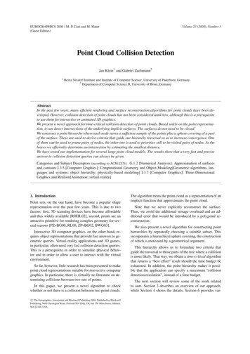
J. Klein and G. Zachmann / Point Cloud Collision Detection# cloud points# sample pointsavg. depth of a nodeSharanHappy 14Table 1: Comparison of the number of cloud points and sample points as well as the average depth of a node in the hierarchy(only objects with appreciably different values are listed).means, we need 32 4(c1 c2 ) bytes for each node. In practice, c1 c2 is between 15 and 30 so that at most 150 bytesper node is needed. For example, the hierarchy of our largestmodel (the grid) consisting of about 65,000 nodes consumesabout 9 MB main memory. Of course, we also have to storethe cloud points in main memory. Table 1 gives an overviewof the number of generated sample points as well as the average depth of a node in the hierarchy.hierarchy construction120time / sec.100806040200050000100000150000# cloud points200000Figure 8: This plot shows the build time of our point cloudhierarchies for various objects.The second step is possible because B λI is positivesemi-definite (because λ is the smallest of all eigenvalues).Thus, the Cholesky decomposition can be performed if fullpivoting is done [Hig90].In our experience, this method is faster than the Jacobimethod by a factor of 4, and it is faster than singular valuedecomposition by a factor 8.6. ResultsWe implemented our new algorithm in C . As of yet, theimplementation is not fully optimized. In the following, allresults have been obtained on a 2.8 GHz Pentium-IV.For timing the performance and measuring the quality, wehave used a set of objects (see Fig. 13), most of them withvarying complexities (with respect to the number of points).Benchmarking is performed by the procedure proposed in[Zac02], which computes average collision detection timesfor a range of distances between two identical objects.6.1. Hierarchy ConstructionOur point cloud hierarchies can be built in a fairly short time,so that the construction can be performed at startup time (seeFig. 8).The memory consumption of a hierarchy is fairly low:with each node, we store a BV, a pointer to the child nodes,1 float for the radius rA , a constant number c1 of pointers tothe sample or to the cloud points lying in A, and also a number c2 of pointers to points in the rε -border of the BV. Thatc The Eurographics Association and Blackwell Publishing 2004.6.2. Time and QualityEach plot in Fig. 9 (left) and Fig. 10 (left) shows the averageruntime for a model of our test suite, which is in the range0.5–2.5 millisec (the two artificial models are consideredlater in this section). This makes our new algorithm suitable for real-time applications, and, in particular, physicallybased simulation in interactive applications. Using our timecritical approach (see Section 5.4), the detection time can bedecreased even further (e.g., when there are too many collisions going on).For each object of our test suite, we have also comparedthe outcome of our new algorithm with a traditional polygonal collision detection using a very high-resolution polygonal model. That way, we can give some experimental hintsabout the error probability of our new algorithm. Note thatthe polygonal models are not a tessellation of the true implicit surface, but just a tessellation of the given point cloud.The results in Fig. 9 (right) and Fig. 10 (right) show that thedifference is always relatively low on average. For distancesbetween 0.6 and 2 about 1.2% (happy buddha), 1.06%(elephant), 1.20% (aphrodite) and 0.64% (sharan) different answers are reported. Here, only collision tests were considered where at least the root BVs intersect. The differencescan be explained by two facts: first implicit surface definedby the vertices of a polygonal object is obviously differentfrom the polygonal model. Second, our intersection findingalgorithm in the leaf nodes is very simplistic at the moment.Equivalent measurements for our two artificial models canbe found in Fig. 11. Note that the models have boundaries,and that the spheres model consists of several unconnectedcomponents. Obviously, our approach achieves results asgood as for the other models. The grid model causes moredifferences compared to polygonal collision detection (up to10%). Probably, this is because the surface definition in Section 4.1 is valid only for manifold objects.

J. Klein and G. Zachmann / Point Cloud Collision Detectiondifference to polygonal collision detection (various objects)timings (various objects)Buddh

erarchy stores a sample of all cloud points lying in A or its rε-border. These sample points are denoted as P A 0 (P A 0 P ). Definition 3 (Test point) A test point is an arbitrary point that is not necessarily contained in a given point cloud. 4.1. Surface Definition We define the surface of a point cloud implicitly based on weighted .