Transcription
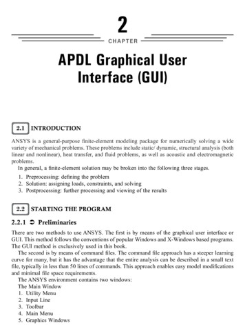
2CHAPTERAPDL Graphical UserInterface (GUI)2.1 INTRODUCTIONANSYS is a general-purpose finite-element modeling package for numerically solving a widevariety of mechanical problems. These problems include static/ dynamic, structural analysis (bothlinear and nonlinear), heat transfer, and fluid problems, as well as acoustic and electromagneticproblems.In general, a finite-element solution may be broken into the following three stages.1. Preprocessing: defining the problem2. Solution: assigning loads, constraints, and solving3. Postprocessing: further processing and viewing of the results2.2 STARTING THE PROGRAM2.2.1 PreliminariesThere are two methods to use ANSYS. The first is by means of the graphical user interface orGUI. This method follows the conventions of popular Windows and X-Windows based programs.The GUI method is exclusively used in this book.The second is by means of command files. The command file approach has a steeper learningcurve for many, but it has the advantage that the entire analysis can be described in a small textfile, typically in less than 50 lines of commands. This approach enables easy model modificationsand minimal file space requirements.The ANSYS environment contains two windows:The Main Window1. Utility Menu2. Input Line3. Toolbar4. Main Menu5. Graphics Windows
APDL Graphical User Interface (GUI)152.2.2 Saving and Restoring JobsIt is a good practice to save the model at various stages during its creation. Very often the stagein the modeling is reached where things have gone well and the model ought to be saved at thispoint. In that way, if mistakes are made later on, it will be possible to come back to this point.To save the model, from ANSYS Utility Menu Select, File - Save as Jobname.db. Themodel will be saved in a file called Jobname.db, where Jobname is the name that was specifiedin the Launcher when ANSYS was first started. It is a good idea to save the job at different timesthroughout the building and analysis of the model to backup the work in case of a system crashor other unforeseen problems.1. Select appropriate drive2. Give the file a name.3. Click OK buttonFigure 2.3Alternatively, select File - Save as.Frequently there is a need to start up ANSYS and recall and continue a previous job. Thereare two methods to do this:1. Using the Launcher.1. In the ANSYS Launcher, select Interactive and specify the previously defined jobname.2. When ANSYS is running, select Utility Menu:File: Resume Jobname.db. This will restore as much of the database (geometry, loads,solution, etc.) as was previously saved.2. Start ANSYS and select Utility Menu: File- Resume from and click on the job fromthe list that appears.1. Select appropriate file from the list2. Click OK button to resume the analysis.
16 Working with ANSYS: A Tutorial ApproachFigure 2.42.2.3 Organization of FilesA large number of files are created when ANSYS is run. If ANSYS is started without specifyinga jobname, the name of all files created will be File.*, where the * represents various extensionsdescribed below. If a jobname is specified, say Pipe, then the created files will all have the fileprefix, Pipe, again with various extensions: pipe.db – database file (binary). This file stores thegeometry, boundary conditions, and any solutions.pipe.dbb: backup of the database file (binary).pipe.err: error file (text). Listing of all error and warning messages.pipe.out: output of all ANSYS operations (text). This is what normally scrolls in the outputwindow during ANSYS session.pipe.log: log file or listing of ANSYS commands (text). Listing of all equivalent ANSYScommand line commands used during the current session.2.2.4 Printing and PlottingANSYS produces lists and tables of many types of results that are normally displayed on thescreen. However, it is often desired to save the results to a file to be later analyzed or includedin a report.In case of stresses, instead of using Plot Results to plot the stresses choose List Results inthe same way as described above. When the list appears on the screen in its own window, select
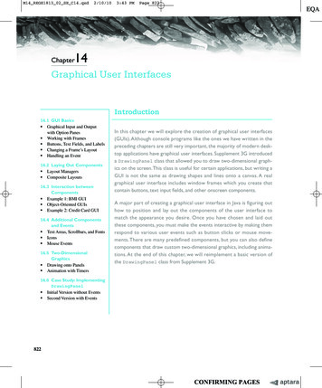
18 Working with ANSYS: A Tutorial Approach5. Select any of the working units6. Click OKFigure 2.62.3.2 Defining Element Types and Real ConstantsThe ANSYS element library contains more than 100 different element types. Each element typehas a unique number and a prefix that identifies the element category.In order to define element types, one must be in PREP7.1.2.3.4.Go to Main Menu- PreprocessorSelect Element TypeGo to Add/Edit/DeleteClick Add Element real constants are properties that depend on the element type, such as cross-sectionalproperties of a beam element. As with element types, each set of real constant has a referencenumber and the table of reference number versus real constant set is called the real constanttable. Not all element types require real constant, and different elements of the same type mayhave different real constant values.1.2.3.4.5.Go to Main Menu - PreprocessorGo to ModelingGo to CreateSelect ElementsSelect Elem Attributes.
APDL Graphical User Interface (GUI)19Figure 2.7Figure 2.82.3.3 Defining Material PropertiesMaterial properties are required for most element types. Depending on the application, materialproperties may be linear or nonlinear, isotropic, orthotropic or anisotropic, constant temperatureor temperature dependent. As with element types and real constants, each set of materialproperties has a material reference number.
20 Working with ANSYS: A Tutorial ApproachThe table of material reference numbers versus material property sets is called the materialtable. In one analysis there may be multiple material property sets corresponding with multiplematerials used in the model. Each set is identified with a unique reference number. Althoughmaterial properties can be defined separately for each finite-element analysis, the ANSYSprogram enables storing a material property set in an archival material library file, then retrievingthe set and reusing it in multiple analyses. Each material property set has its own library file.The material library files also make it possible for several users to share commonly used materialproperty data.1.2.3.4.5.Go to ANSYS Main Menu - PreprocessorSelect Material PropsSelect Material ModelsProvide a material ID numberSelect from the available sets of modelFigure 2.92.3.4 Construction of the ModelOnce material properties are defined, the next step in an analysis is generating a finite elementmodel – nodes and element adequately describing the model geometry. There are two methodsto create the finite-element model: solid modeling and direct generation.With solid modeling, the geometry of shape of the model is described, and then the ANSYSprogram automatically meshes the geometry with nodes and elements. The size and shape of theelements that the program creates can be controlled. With direct generation, the location of eachnode and the connectivity of each element is manually defined. Several convenience operations,such as copying patterns of existing nodes and elements, symmetry reflection, etc., are available.
22 Working with ANSYS: A Tutorial ApproachUsing this postprocessor contour displays, deformed shapes, and tabular listings to reviewand interpret the results of the analysis can be obtained. POST1 offers many othercapabilities, including error estimation, load case combinations, calculations among resultsdata, and path operations. POST26: The time history postprocessor is used to review results at specific points in themodel over all time steps. The commandto enter POST26 is as follows: from ANSYSMain Menu select Time Hist Postprocessor. Graph plots of results data versus time(or frequency) and tabular listings can be obtained. Other POST26 capabilities includearithmetic calculations and complex algebra.
APDL Graphical User Interface (GUI)15 2 . 20 Working with ANSYS: A Tutorial Approach The table of material reference numbers versus material property sets is called the material table. In one analysis there may be multiple material property sets corresponding with multiple materials used in the model. Each set is identified with a unique reference number. Although material properties can be .