Transcription
Conditional Value-at-Risk (CVaR):Algorithms and ApplicationsStan UryasevRisk Management and Financial Engineering LabUniversity of Floridae-mail: uryasev@ise.ufl.eduhttp://www.ise.ufl.edu/uryasev
OUTLINE OF PRESENTATION Background: percentile and probabilistic functions inoptimization Definition of Conditional Value-at-Risk (CVaR) and basicproperties Optimization and risk management with CVaR functions Case studies: Definition of Conditional Drawdown-at-Risk (CDaR) Conclusion
PAPERS ON MINIMUM CVAR APPROACHPresentation is based on the following papers:[1] Rockafellar R.T. and S. Uryasev (2001): Conditional Value-atRisk for General Loss Distributions. Research Report 2001-5. ISEDept., University of Florida, April 2001.(download: www.ise.ufl.edu/uryasev/cvar2.pdf)[2] Rockafellar R.T. and S. Uryasev (2000): Optimization ofConditional Value-at-Risk. The Journal of Risk. Vol. 2, No. 3, 2000,21-41 (download: www.ise.ufl.edu/uryasev/cvar.pdf)Several more papers on applications of Conditional Value-at-Riskand the related risk measure, Conditional Drawdown-at-Risk, canbe downloaded from www.ise.ufl.edu/rmfe
ABSTRACT OF PAPER1“Fundamental properties of Conditional Value-at-Risk (CVaR), as ameasure of risk with significant advantages over Value-at-Risk,are derived for loss distributions in finance that can involvediscreetness. Such distributions are of particular importance inapplications because of the prevalence of models based onscenarios and finite sampling. Conditional Value-at-Risk is able toquantify dangers beyond Value-at-Risk, and moreover it iscoherent. It provides optimization shortcuts which, through linearprogramming techniques, make practical many large-scalecalculations that could otherwise be out of reach. The numericalefficiency and stability of such calculations, shown in severalcase studies, are illustrated further with an example of indextracking.”1RockafellarR.T. and S. Uryasev (2001): Conditional Value-at-Risk for General Loss Distributions.Research Report 2001-5. ISE Dept., University of Florida, April 2001.(download: www.ise.ufl.edu/uryasev/cvar2.pdf)
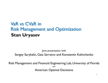
PERCENTILE MEASURES OF LOSS (OR REWARD) Let f(x,y) be a loss functions depending upon a decision vectorx ( x1 , , xn ) and a random vector y ( y1 , , ym ) VaR α percentile of loss distribution (a smallest value such thatprobability that losses exceed or equal to this value isgreater or equal to α ) CVaR ( “upper CVaR” ) expected losses strictly exceeding VaR(also called Mean Excess Loss and Expected Shortfall) CVaR- ( “lower CVaR” ) expected losses weakly exceeding VaR,i.e., expected losses which are equal to or exceed VaR(also called Tail VaR) CVaR is a weighted average of VaR and CVaR CVaR λ VaR (1- λ) CVaR ,0 λ 1
Fre q ue n cyVaR, CVaR, CVaR and CVaR-MaximumlossVaRProbability1 αCVaRLoss
CVaR: NICE CONVEX FUNCTIONCVaR RiskCVaRCVaRVaRxCVaR is convex, but VaR, CVaR- ,CVaR may be non-convex,inequalities are valid: VaR CVaR- CVaR CVaR
VaR IS A STANDARD IN FINANCE Value-at-Risk (VaR) is a popular measure of risk:current standard in finance industryvarious resources can be found at http://www.gloriamundi.org Informally VaR can be defined as a maximum loss in aspecified period with some confidence level (e.g.,confidence level 95%, period 1 week) Formally, α VaR is the α percentile of the lossdistribution:α VaR is a smallest value such that probability that loss exceedsor equals to this value is bigger or equals to α
FORMAL DEFINITION OF CVaR Notations:Ψ cumulative distribution of losses,Ψα α-tail distribution, which equals to zero for losses below VaR,and equals to (Ψ- α)/(1 α) for losses exceeding or equal to VaRDefinition:CVaR is mean of α-tail distribution Ψα11α Ψα(ζ)Ψ(ζ)αα α α1 α0VaRζCumulative Distribution of Losses, Ψ0VaRα-Tail Distribution, Ψαζ
CVaR: WEIGHTED AVERAGE Notations:VaR α percentile of loss distribution (a smallest value such thatprobability that losses exceed or equal to this value is greater orequal to α )CVaR ( “upper CVaR” ) expected losses strictly exceeding VaR(also called Mean Excess Loss and Expected Shortfall)Ψ(VaR) probability that losses do not exceed VaR or equal to VaRλ (Ψ(VaR) - α)/ (1 α) ,( 0 λ 1 ) CVaR is weighted average of VaR and CVaR CVaR λ VaR (1- λ) CVaR
CVaR: DISCRETE DISTRIBUTION, EXAMPLE 1 α does not “split” atoms: VaR CVaR- CVaR CVaR ,λ (Ψ- α)/ (1 α) 0Six scenarios,p1 p2 L p6 16 , α 23 46CVaR CVaR 12 f 5 12 f 6CVaRProbability16f1Loss16f2161616f4f3VaR16f5CVaR --f6CVaR
CVaR: DISCRETE DISTRIBUTION, EXAMPLE 2 α “splits” the atom: VaR CVaR- CVaR CVaR ,λ (Ψ- α)/ (1 α) 0Six scenarios,p1 p 2 L p 6 16 , α CVaR 15 VaR 54 CVaR 15f4 f1f5 aRCVaR--1216f6f5 12 f6 CVaR
CVaR: DISCRETE DISTRIBUTION, EXAMPLE 3 α “splits” the last atom: VaR CVaR- CVaR,CVaR is not defined, λ (Ψ α)/ (1 α) 0Four scenarios, p1 p2 p3 p4 14 , α 87CVaR VaR f 4CVaRProbability14f1Loss141414f2f3f4VaR18
CVaR: NICE CONVEX FUNCTIONCVaR RiskCVaRCVaRVaRPositionCVaR is convex, but VaR, CVaR- ,CVaR may be non-convex,inequalities are valid: VaR CVaR- CVaR CVaR
CVaR FEATURES1,2- simple convenient representation of risks (one number)- measures downside risk- applicable to non-symmetric loss distributions- CVaR accounts for risks beyond VaR (more conservative than VaR)- CVaR is convex with respect to portfolio positions- VaR CVaR- CVaR CVaR - coherent in the sense of Artzner, Delbaen, Eber and Heath3:(translation invariant, sub-additive, positively homogeneous, monotonicw.r.t. Stochastic Dominance1)1RockafellarR.T. and S. Uryasev (2001): Conditional Value-at-Risk for General Loss Distributions.Research Report 2001-5. ISE Dept., University of Florida, April 2001. (Can be g, G. Some Remarks on the Value-at-Risk and the Conditional Value-at-Risk, in ProbabilisticConstrained Optimization: Methodology and Applications'' (S. Uryasev ed.), Kluwer AcademicPublishers, 2001.3Artzner,P., Delbaen, F., Eber, J.-M. Heath D. Coherent Measures of Risk, Mathematical Finance, 9(1999), 203--228.
CVaR FEATURES (Cont’d)- stable statistical estimates (CVaR has integral characteristicscompared to VaR which may be significantly impacted by one scenario)- CVaR is continuous with respect to confidence level α ,consistent at different confidence levels compared to VaR( VaR, CVaR-, CVaR may be discontinuous in α )- consistency with mean-variance approach: for normal lossdistributions optimal variance and CVaR portfolios coincide- easy to control/optimize for non-normal distributions;linear programming (LP): can be used for optimizationof very large problems (over 1,000,000 instruments andscenarios); fast, stable algorithms- loss distribution can be shaped using CVaR constraints (many LPconstraints with various confidence levels α in different intervals)- can be used in fast online procedures
CVaR versus EXPECTED SHORTFALL CVaR for continuous distributions usually coincides withconditional expected loss exceeding VaR (also called Mean ExcessLoss or Expected Shortfall). However, for non-continuous (as well as for continuous)distributions CVaR may differ from conditional expected lossexceeding VaR. Acerbi et al.1,2 recently redefined Expected Shortfall to be consistentwith CVaR definition. Acerbi et al.2 proved several nice mathematical results on propertiesof CVaR, including asymptotic convergence of sample estimates toCVaR.1Acerbi,C., Nordio, C., Sirtori, C. Expected Shortfall as a Tool for Financial RiskManagement, Working Paper, can be downloaded: www.gloriamundi.org/var/wps.html2Acerbi,C., and Tasche, D. On the Coherence of Expected Shortfall.Working Paper, can be downloaded: www.gloriamundi.org/var/wps.html
CVaR OPTIMIZATION Notations:x (x1,.xn) decision vector (e.g., portfolio weights)X a convex set of feasible decisionsy (y1,.yn) random vectory j scenario of random vector y , ( j 1,.J )f(x,y) loss functions Example: Two Instrument PortfolioA portfolio consists of two instruments (e.g., options). Let x (x1,x2) be avector of positions, m (m1,m2) be a vector of initial prices, and y (y1,y2) bea vector of uncertain prices in the next day. The loss function equals thedifference between the current value of the portfolio, (x1m1 x2m2), and anuncertain value of the portfolio at the next day (x1y1 x2y2), i.e.,f(x,y) (x1m1 x2m2)–(x1y1 x2y2) x1(m1–y1) x2(m2–y2) .If we do not allow short positions, the feasible set of portfolios is a twodimensional set of non-negative numbersX {(x1,x2), x1 0, x2 0} .Scenarios y j (y j1,y j2), j 1,.J , are sample daily prices (e.g., historicaldata for J trading days).
CVaR OPTIMIZATION (Cont’d) CVaR minimizationmin{ x X } CVaRcan be reduced to the following linear programming (LP) problemmin{ x X , ζ R , z RJ } ζ ν { j 1,.,J } zjsubject tozj f(x,y j) - ζ ,zj 0 , j 1,.J(νν (( 1- α)J)-1 const ) By solving LP we find an optimal portfolio x* , corresponding VaR,which equals to the lowest optimal ζ *, and minimal CVaR, whichequals to the optimal value of the linear performance function Constraints, x X , may account for various trading constraints,including mean return constraint (e.g., expected return shouldexceed 10%) Similar to return - variance analysis, we can construct an efficientfrontier and find a tangent portfolio
RISK MANAGEMENT WITH CVaR CONSTRAINTS CVaR constraints in optimization problems can be replaced by aset of linear constraints. E.g., the following CVaR constraintCVaR Ccan be replaced by linear constraintsζ ν { j 1,.,J } zj Czj f(x,y j) - ζ ,zj 0 , j 1,.J( ν (( 1- α)J)-1 const ) Loss distribution can be shaped using multiple CVaR constraintsat different confidence levels in different times The reduction of the CVaR risk management problems to LP is arelatively simple fact following from possibility to replace CVaR bysome function F (x, ζ) , which is convex and piece-wise linear withrespect to x and ζ . A simple explanation of CVaR optimizationapproach can be found in paper1 .1Uryasev,S. Conditional Value-at-Risk: Optimization Algorithms and Applications.Financial Engineering News, No. 14, February, 2000.(can be downloaded: www.ise.ufl.edu/uryasev/pubs.html#t).
CVaR OPTIMIZATION: MATHEMATICAL BACKGROUNDDefinitionF (x, ζ) ζ ν Σj 1,J ( f(x,y j )- ζ) ,ν (( 1- α)J)-1 constTheorem 1.CVaRα(x) min ζ Rζ F (x, ζ) and ζα(x) is a smallest minimizerRemark. This equality can be used as a definition of CVaR ( Pflug ).Theorem 2.min x X CVaRα(x) min ζ R, X F (x, ζ)ζ x (1) Minimizing of F (x, ζ) simultaneously calculates VaR ζα(x),optimal decision x, and optimal CVaR Problem (1) can be reduces to LP using additional variables
PERCENTILE V.S. PROBABILISTIC CONSTRAINTSProposition 1.Let f(x,y) be a loss functions and ζα(x) be α- percentile (αα-VaR) thenζα(x) εóPr{ f(x,y) ε } αProof follows from the definition of α- percentile ζα(x)ζα(x) min {εε : Pr{ f(x,y) ε } α } Generally, ζα(x) is nonconvex (e.g., discrete distributions),therefore ζα(x) ε as well as Pr( f(x,y) ε ) α may benonconvex constraints Probabilistic constraints were considered by Prekopa, Raik,Szantai, Kibzun, Uryasev, Lepp, Mayer, Ermoliev, Kall, Pflug,Gaivoronski,
NON-PERCENTILE RISK MEASURES Low partial moment constraint (considered in finance literaturefrom 70-th)E{ ((f(x,y) - ε ) )a } b ,a 0, g max{0,g}special casesa 0 Pr{ f(x,y) - ε }a 1 E{ (f(x,y) - ε ) }a 2 , ε E f(x,y) semi-variance E{ ((f(x,y) - ε ) )2 } Regret (King, Dembo) is a variant of low partial moment withε 0 and f(x,y) performance-benchmark Various variants of low partial moment were successfully appliedin stochastic optimization by Ziemba, Mulvey, Zenios,Konno,King, Dembo,Mausser,Rosen, Haneveld and Prekopa considered a special case of low partialmoment with a 1, ε 0: integrated chance constraints
PERCENTILE V.S. LOW PARTIAL MOMENT Low partial moment with a 0 does not control percentiles. It isapplied when loss can be hedged at additional costtotal expected value expected cost without high losses expected cost of high lossesexpected cost of high losses p E{ (f(x,y) - ε ) } Percentiles constraints control risks explicitly in percentile terms. Testury and Uryasev1 established equivalence between CVaRapproach (percentile measure) and low partial moment, a 1 (nonpercentile measure) in the following sense:a) Suppose that a decision is optimal in an optimization problemwith a CVaR constraint, then the same decision is optimal with a lowpartial moment constraint with some ε 0;b) Suppose that a decision is optimal in an optimization problemwith a low partial moment constraint, then the same decision isoptimal with a CVaR constraint at some confidence level α.1Testuri,C.E. and S. Uryasev. On Relation between Expected Regret and Conditional Value-At-Risk.Research Report 2000-9. ISE Dept., University of Florida, August 2000. Submitted to Decisions inEconomics and Finance journal. (www.ise.ufl.edu/uryasev/Testuri.pdf)
CVaR AND MEAN VARIANCE: NORMAL RETURNS
CVaR AND MEAN VARIANCE: NORMAL RETURNSIf returns are normally distributed, and return constraint is active,the following portfolio optimization problems have the samesolution:1. Minimize CVaRsubject to return and other constraints2. Minimize VaRsubject to return and other constraints3. Minimize variancesubject to return and other constraints
EXAMPLE 1: PORTFOLIO MEAN RETURN AND COVARIANCE
OPTIMAL PORTFOLIO (MIN VARIANCE APPROACH)ααα
PORTFOLIO, VaR and CVaR (CVaR APPROACH)α
EXAMPLE 2: NIKKEI PORTFOLIO
NIKKEI PORTFOLIO
HEDGING: NIKKEI PORTFOLIO
HEDGING: MINIM CVaR APPROACH
ONE INSTRUMENT HEDGING
ONE - INSTRUMENT HEDGINGα
MULTIPLE INSTRUMENT HEDGING: CVaR APROACH
MULTIPLE - INSTRUMENT HEDGING
MULTIPLE-HEDGING: MODEL DESCRIPTION
EXAMPLE 3: PORTFOLIO REPLICATION USING CVaR Problem Statement: Replicate an index usingj 1,K, n instruments. Considerimpact of CVaR constraints on characteristics of the replicating portfolio. Daily Data: SP100 index, 30 stocks (tickers: GD, UIS, NSM, ORCL, CSCO, HET, BS,TXN, HM,INTC, RAL, NT, MER, KM, BHI, CEN, HAL, DK, HWP, LTD, BAC, AVP, AXP, AA, BA, AGC, BAX, AIG, AN, AEP) NotationsIt price of SP100 index at times t 1,K,Tp j t prices of stocks j 1,K, n at times t 1,K,Tν amount of money to be on hand at the final time Tθ νIT number of units of the index at the final time Tx j number of units of j-th stock in the replicating portfolioDefinitions (similar to paper1 ) n pj 1jtx j value of the portfolio at time tn (θ It p j t x j ) /(θ It ) absolute relative deviation of the portfolio from the target θ Itj 1nf ( x, pt ) ( θ It p j t x j ) /(θ It ) relative portfolio underperformance compared to target at time tj 11KonnoH. and A. Wijayanayake. Minimal Cost Index Tracking under Nonlinear Transaction Costs andMinimal Transaction Unit Constraints,Tokyo Institute of Technology, CRAFT Working paper 00-07,(2000).
PORTFOLIO REPLICATION (Cont’d)Portfolio value 01 151 201 251 301 351 401 451 501 551Day number: in-sample regionIndex and optimal portfolio values in in-sample region, CVaRconstraint is inactive (w 0.02)
PORTFOLIO REPLICATION 91857973676155494337312519138500790001Portfolio value (USD)11500Day number in out-of-sample regionIndex and optimal portfolio values in out-of-sample region,CVaR constraint is inactive (w 0.02)
PORTFOLIO REPLICATION (Cont’d)Portfolio value 40135130125120115110151012000Day number: in-sample regionIndex and optimal portfolio values in in-sample region,CVaR constraint is active (w 0.005).
PORTFOLIO REPLICATION (Cont’d)12000Portfolio value 973676155494337312519137850019000Day number in out-of-sample regionIndex and optimal portfolio values in out-of-sample region,CVaR constraint is active (w 0.005).
PORTFOLIO REPLICATION (Cont’d)32Discrepancy (%)10-1activeinactive-2-3-4-5-6151 101 151 201 251 301 351 401 451 501 551Day number: in-sample regionRelative underperformance in in-sample region, CVaRconstraint is active (w 0.005) and inactive (w 0.02).
PORTFOLIO REPLICATION (Cont’d)65Discrepancy (%)43activeinactive210-1-216 11 16 21 26 31 36 41 46 51 56 61 66 71 76 81 86 91 96Day number in out-of-sample regionRelative underperformance in out-of-sample region, CVaRconstraint is active (w 0.005) and inactive (w 0.02)
PORTFOLIO REPLICATION (Cont’d)65in -s a m p le o b je c tiv ef u n c tio no u t- o f -s a m p le o b je c tiv ef u n c tio no u t- o f -s a m p le C V A RValue (%)432100 .0 20 .0 10 .0 0 50 .0 0 30 .0 0 1om egaIn-sample objective function (mean absolute relative deviation),out-of-sample objective function, out-of-sample CVaR for variousrisk levels w in CVaR constraint.
PORTFOLIO REPLICATION (Cont’d) Calculation resultsC VaRin -sam p le (600 d ays)ou t -of-sa m p le ( 100 d ays)ou t -of-sam p le C VaRlevel wob ject ive fu n ct ion , in %ob ject ive fu n ct ion , in %in 9960.0011.481240.800781.88564 CVaR constraint reduced underperformance of the portfolio versus the index both inthe in-sample region (Column 1 of table) and in the out-of-sample region (Column 4) .For w 0.02, the CVaR constraint is inactive, for w 0.01, CVaR constraint is active. Decreasing of CVaR causes an increase of objective function (mean absolutedeviation) in the in-sample region (Column 2). Decreasing of CVaR causes a decrease of objective function in the out-of-sampleregion (Column 3). However, this reduction is data specific, it was not observed forsome other datasets.
PORTFOLIO REPLICATION (Cont’d)In-sample-calculations: w 0.005 Calculations were conducted using custom developed software (C ) in combinationwith CPLEX linear programming solver For optimal portfolio, CVaR 0.005. Optimal ζ * 0.001538627671 gives VaR. Probabilityof the VaR point is 14/600 (i.e.14 days have the same deviation 0.001538627671). Thelosses of 54 scenarios exceed VaR. The probability of exceeding VaR equals54/600 1- α , andλ (Ψ(VaR) - α) / (1 - α) [546/600 - 0.9]/[1 - 0.9] 0.1 Since α “splits” VaR probability atom, i.e., Ψ(VaR) - α 0, CVaR is bigger than CVaR(“lower CVaR”) and smaller than CVaR ( “upper CVaR”, also called expected shortfall)CVaR- 0.004592779726 CVaR 0.005 CVaR 0.005384596925 CVaR is the weighted average of VaR and CVaR CVaR λ VaR (1- λ) CVaR 0.1 * 0.001538627671 0.9 * 0.005384596925 0.005 In several runs, ζ* overestimated VaR because of the nonuniqueness of the optimalsolution. VaR equals the smallest optimal ζ*.
EXAMPLE 4: CREDIT RISK (Related Papers) Andersson, Uryasev, Rosen and Mausser applied the CVaRapproach to a credit portfolio of bonds– Andersson, F., Mausser, Rosen, D. and S. Uryasev (2000),“Credit risk optimization with Conditional Value-at-Risk criterion”,Mathematical Programming, series B, December) Uryasev and Rockafellar developed the approach to minimizeConditional Value-at-Risk– Rockafellar, R.T. and S. Uryasev (2000), ”Optimization of ConditionalValue-at-Risk”, The Journal of Risk, Vol. 2 No. 3 Bucay and Rosen applied the CreditMetrics methodology toestimate the credit risk of an international bond portfolio– Bucay, N. and D. Rosen, (1999)“Credit risk of an international bondportfolio: A case study”, Algo Research Quarterly, Vol. 2 No. 1, 9-29 Mausser and Rosen applied a similar approach based on theexpected regret risk measure– Mausser, H. and D. Rosen (1999), “Applying scenario optimization toportfolio credit risk”, Algo Research Quarterly, Vol. 2, No. 2, 19-33
Basic Definitions Credit risk– The potential that a bank borrower or counterpart will fail tomeet its obligations in accordance with agreed terms Credit loss– Losses due to credit events, including both default and creditmigration
FrequencyCredit Risk MeasuresAllocated economic capitalUnexpected loss (95%)(Value-at-Risk (95%))Conditional Value-at-Risk (95%)Expected lossTarget insolvency rate 5%Credit lossCVaR
Bond Portfolio Compiled to asses to the state-of-the-art portfolio credit riskmodels Consists of 197 bonds, issued by 86 obligors in 29countries Mark-to-market value of the portfolio is 8.8 billions of USD Most instruments denominated in USD but 11 instrumentsare denominated in DEM(4), GBP(1), ITL(1), JPY(1), TRL(1),XEU(2) and ZAR(1) Bond maturities range from a few months to 98 years,portfolio duration of approximately five years
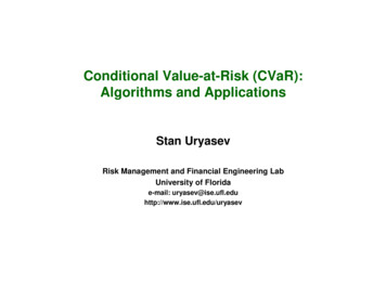
Portfolio Loss Distribution1000500Portfolio loss (millions of USD)2388212518631600133710758125490286 Standard deviation of 232 MUSDVaR (99%) equal 1026 M USDCVaR (99%) equal 1320 MUSD150024 2000-239– Only credit losses, nointerest income2500-502 Generated by a Monte Carlosimulation based on 20000scenariosSkewed with a long fat tailExpected loss of 95 M USDFrequency
Model Parameters Definitions– 1) Obligor weights expressed as multiples of current holdings– 2) Future values without credit migration, i.e. the benchmarkscenario– 3) Future scenario dependent values with credit migration– 4) Portfolio loss due to credit migration(Instrument positions) x ( x1 , x2 ,., xn ) (1)(Future values without credit migration) b (b1 , b2 ,., bn ) (2)(Future values with credit migration) y ( y1 , y2 ,., yn ) (3)(Portfolio loss) f ( x, y ) (b y )T x (4)
OPTIMIZATION PROBLEMMinimize1α (1 β ) JJ zjj 1Subject to :(Excess loss)nz j ((bi y j , i ) xi ) α ,j 1,., J ,z j 0,j 1,., J ,li xi u i ,i 1,., n,i 1(Upper/low er bound)(Portfolio value)(Expected return)nni 1i 1 q i xi q i ,n qi (ri R ) xi 0,i 1( Long position)nxi qi 0,20 qi ,i 1i 1,., n
SINGLE - INSTRUMENT OPTIMIZATIONObligorBest HedgeVaR (M USD)VaR (%)CVaR (M USD)CVaR 8312922Philippines-3.241015113091
MULTIPLE - INSTRUMENT OPTIMIZATIONVaR and CVaR (millions of USD)25002000Original VaR1500No Short VaRLong and Short VaROriginal CVaRNo Short CVaR1000Long and Short CVaR5000909599Percentile level(%)99.9
RISK CONTRIBUTION (original PeruMarginal CVaR (%)3530BrazilRussia2520PanamaMoscow TelMulticanalMoroccoArgentina15Globo Romania Credit exposure (millions of USD)7008009001000
RISK CONTRIBUTION (optimized portfolio)504540Marginal risk (%)3530252015Romania10 gentinaBulgariaMexicoKazakhstanSlovakia00Moscow TelKorea JordanTelefarg200Croatia300South ael500Credit exposure (millions of USD)600700800
EFFICIENT FRONTIER16Portfolio return (%)1412VaRCVaROriginal VaR10Original CVaROriginal Return87,62102613206402004006008001000Conditional Value-at-Risk (99%) (millions of USD)12001400
CONDITIONAL DRAWDOWN-AT-RISK (CDaR) CDaR1 is a new risk measure closely related to CVaRDrawdown is defined as a drop in the portfolio value compared tothe previous maximum CDaR is the average of the worst z% portfolio drawdowns observedin the past (e.q., 5% of worst drawdowns). Similar to CVaR,averaging is done using α-tail distribution. Notations:w(x,t ) uncompounded portfolio valuet timex (x1,.xn) portfolio weightsf (x,t ) max{ 0 τ t } [w(x,τ )] - w(x,t ) drawdown Formal definition:CDaR is CVaR with drawdown loss function f (x,t ) . CDaR can be controlled and optimized using linear programmingsimilar to CVaR Detail discussion of CDaR is beyond the scope of this presentation1Chekhlov,A., Uryasev, S., and M. Zabarankin. Portfolio Optimization with DrawdownConstraints. Research Report 2000-5. ISE Dept., University of Florida, April 2000.
CDaR: EXAMPLE GRAPHReturn and Drawdown0.0070.0060.0050.0040.0030.0020.001time (working days)Rate of ReturnDrawDown function35333129272523211917151311975310
CONCLUSION CVaR is a new risk measure with significant advantages comparedto VaR- can quantify risks beyond VaR- coherent risk measure- consistent for various confidence levels α ( smooth w.r.t α )- relatively stable statistical estimates (integral characteristics) CVaR is an excellent tool for risk management and portfoliooptimization- optimization with linear programming: very large dimensions and stablenumerical implementations- shaping distributions: multiple risk constraints with differentconfidence levels at different times- fast algorithms which can be used in online applications, such as activeportfolio management CVaR methodology is consistent with mean-variancemethodology under normality assumption- CVaR minimal portfolio (with return constraint) is also variance minimalfor normal loss distributions
CONCLUSION (Cont’d) Various case studies demonstrated high efficiency andstability of of the approach (papers can be downloaded:www.ise.ufl.edu/uryasev)- optimization of a portfolio of stocks- hedging of a portfolio of options- credit risk management (bond portfolio optimization)- asset and liability modeling- portfolio replication- optimal position closing strategies CVaR has a great potential for further development. It stimulatedseveral areas of applied research, such as Conditional Drawdownat-Risk and specialized optimization algorithms for riskmanagement Risk Management and Financial Engineering Lab at UF(www.ise.ufl.edu/rmfe) leads research in CVaR methodology andis interested in applied collaborative projects
APPENDIX: RELEVANT PUBLICATIONS[1] Bogentoft, E. Romeijn, H.E. and S. Uryasev (2001): Asset/Liability Management forPension Funds Using Cvar Constraints. Submitted to The Journal of Risk Finance(download: www.ise.ufl.edu/uryasev/multi JRB.pdf)[2] Larsen, N., Mausser H., and S. Uryasev (2001): Algorithms For Optimization OfValue-At-Risk . Research Report 2001-9, ISE Dept., University of Florida, August, 2001(www.ise.ufl.edu/uryasev/wp VaR minimization.pdf)[3] Rockafellar R.T. and S. Uryasev (2001): Conditional Value-at-Risk for General LossDistributions. Submitted to The Journal of Banking and Finance (relevantResearch Report 2001-5. ISE Dept., University of Florida, April 2001,www.ise.ufl.edu/uryasev/cvar2.pdf)[4] Uryasev, S. Conditional Value-at-Risk (2000): Optimization Algorithms andApplications. Financial Engineering News, No. 14, February, 2000.(www.ise.ufl.edu/uryasev/finnews.pdf )[5] Rockafellar R.T. and S. Uryasev (2000): Optimization of Conditional Value-at-Risk.The Journal of Risk. Vol. 2, No. 3, 2000, 21-41.( www.ise.ufl.edu/uryasev/cvar.pdf).[6] Andersson, F., Mausser, H., Rosen, D., and S. Uryasev (2000): Credit RiskOptimization With Conditional Value-At-Risk Criterion. Mathematical Programming,Series B, December, 2000.(/www.ise.ufl.edu/uryasev/Credit risk optimization.pdf)
APPENDIX: RELEVANT PUBLICATIONS (Cont’d)[7] Palmquist, J., Uryasev, S., and P. Krokhmal (1999): Portfolio Optimization withConditional Value-At-Risk Objective and Constraints. Submitted to The Journal ofRisk (www.ise.ufl.edu/uryasev/pal.pdf)[8] Chekhlov, A., Uryasev, S., and M. Zabarankin (2000): Portfolio Optimization WithDrawdown Constraints. Submitted to Applied Mathematical Finance journal.(www.ise.ufl.edu/uryasev/drd 2000-5.pdf)[9] Testuri, C.E. and S. Uryasev. On Relation between Expected Regret andConditional Value-At-Risk. Research Report 2000-9. ISE Dept., University of Florida,August 2000. Submitted to Decisions in Economics and Finance journal.(www.ise.ufl.edu/uryasev/Testuri.pdf)[10] Krawczyk, J.B. and S. Uryasev. Relaxation Algorithms to Find Nash Equilibriawith Economic Applications. Environmental Modeling and Assessment, 5, 2000, 6373. .pdf)[11] Uryasev, S. Introduction to the Theory of Probabilistic Functions and Percentiles(Value-at-Risk). In “Probabilistic Constrained Optimization: Methodology andApplications,” Ed. S. Uryasev, Kluwer Academic Publishers, 2000.(www.ise.ufl.edu/uryasev/intr.pdf).
APPENDIX: BOOKS[1] Uryasev, S. Ed. “Probabilistic Constrained Optimization:Methodology and Applications,” Kluwer AcademicPublishers, 2000.[2] Uryasev, S. and P. Pardalos, Eds. “ StochasticOptimization: Algorithms and Applications,” KluwerAcademic Publishers, 2001 (proceedings of the conferenceon Stochastic Optimization, Gainesville, FL, 2000).
A portfolio consists of two instruments (e.g., options). Let x (x1,x2) be a vector of positions, m (m1,m2)be a vector ofinitial prices, and y (y1,y2) be a vector of uncertain prices in the next day. The loss function equals the . Constraints, x X , may account for various trading constraints, including mean return constraint (e.g .