Transcription
Highline Excel 2016 Class 16: Conditional Formatting to Visualize DataTable of ContentsConditional Formatting . 2Apply Conditional Formatting: . 2Built-in features to Conditional Formatting . 3Logical Formulas: . 4Steps in Creating Conditional Formatting with Formulas: . 4Conditional Formatting is Volatile: it Recalculates Often and can Slow Overall Spreadsheet Calculation Time. . 5Example 1: Built-in Feature: Cell Contains . 6Visual Steps for using Built-in Conditional Formatting Feature . 6Example 2: Logical Formula: Highlight Row (Record) where cell contains a value. 7Visual Steps for Conditional Formatting with a Formula. . 7Example 3: Built-in Feature: Below Average. 9Example 4: Logical Formula: Highlight Row (Record) where sales are below average. . 9Example 5: Built-in Feature: Top 3 values. 10Example 6: Logical Formula: Highlight Records that contain the top 3 values . 10Example 7: Built-in Feature: Data Bars . 11Example 8: Built-in Feature: Color Scales (Heat Map) . 11Example 9: Built-in Feature: Icons . 12Example 10: Logical Formula: Format Whole Column Based on a condition . 12Example 11: Logical Formula: Format with complex criteria (AND Logical Test) . 13Example 12: Logical Formula: Format with complex criteria (OR Logical Test) . 13Example 13: Logical Formula: Format Weekends and Holidays . 14Example 14: Logical Formula: Format items NOT in List . 15Further Reference for Conditional Formatting: . 15Cumulative List of Keyboards Throughout Class:. 16Page 1 of 17
Conditional Formatting1) Conditional Formatting for cells in a highlighted range requires a logical test that comes out TRUE orFALSE. TRUE Cell gets Formatting. FALSE Cell NOT get Formatting.2) Conditional Formatting can be applied to cells with: Built-in features like:1. Contains a value2. Top 3 values3. Above Average4. Data Bars5. Color Scales (Heat Map)6. Icons Logical Formulas:1. Highlight Row (Record) where cell contains a value.2. Highlight Row (Record) where sales are below average.3. Highlight Records that contain the top 3 values.4. Format Whole Column Based on a condition.5. Format with complex criteria (AND Logical Test).6. Format with complex criteria (OR Logical Test).7. Format Weekends and Holidays.8. Format items NOT in List.Apply Conditional Formatting:1) Home Ribbon Tab, Styles group, Conditional Formatting button:2) Keyboards: Keyboard for New Format Rule dialog box:Alt, H, L, N Keyboard for Manage Rule dialog box:Alt, O, D Keyboard to delete rule:Alt, O, D, D, Enter Keyboard to get to “Format values where this formula is true”:1. Alt, H, L, N, PageDown, TabPage 2 of 17
Built-in features to Conditional FormattingSteps:1) Highlight cells2) Home Ribbon Tab, Styles group, Conditional Formatting button3) Select Rule4) Choose formattingBuilt-in Conditional Formatting Options:Page 3 of 17
Logical Formulas:1) Logical Formulas are formulas that evaluate to TRUE or FALSE2) For Conditional Formatting: Formatting IS Applied when the formula evaluates to:1. TRUE2. Any non-zero number Formatting is NOT Applied when the formula evaluates to:1. FALSE2. Zero3. Error3) When you use Logical Formulas to apply Conditional Formatting: Formula has to calculate in every cell in the range!!! Rule to minimize calculation time:1. Choose formulas that calculate quickly.2. Use Helper Cells for sub-calculations so that the Conditional Formatting Logical Formuladon’t have to run the sub-calculation in every cell in the Conditional Formatting range.4) Array Formulas work in the Conditional Formatting dialog box (without using Ctrl Shift Enter), butshould be avoided if overall spreadsheet calculation time is an issue.Steps in Creating Conditional Formatting with Formulas:1) Highlight the range of cells. Make a metal note of which cell is the active cell in the highlighted2) range. (The active cell is the light-colored cell.)3) Open the Conditional Formatting Rules Manager dialog (from the Home Ribbon tab, select the Stylesgroup and then select Manage Rules from the Conditional Formatting drop-down).4) Open the New Formatting Rule dialog box (by clicking the New Rule button).5) Select Use a Formula to Determine Which Cells to Format from the "Select a Rule Type" list.6) Click the Format Values Where This Formula Is True text box.7) Create your formula from the point of view of the active cell in the highlighted range. That is, build theformula as if you were placing it into the active cell and then copying it down and over. Remember,whatever the conditional test is that you are creating must be evaluated for each cell to determinewhether each cell in the range gets the formatting. So, even if the formula is not actually going into theactive cell, the dialog box will copy it throughout the range in memory as if the formula were in the cellsin the highlighted range.8) Click the Format button and select any combination of formatting you want from the four tabs (Number,Font, Border, and Fill).9) Click OK in the Format Cells dialog box.10) Click OK in the New Formatting Rule dialog box.11) Click OK in the Conditional Formatting Rules Manager dialog box.Page 4 of 17
Conditional Formatting is Volatile: it Recalculates Often and can Slow Overall SpreadsheetCalculation Time.1) Conditional Formatting is recalculated for cells that are visible on the screen Large screens have more cells to calculate than small screens. Zoomed out has more cells to calculate than zoomed in. Scrolling up or down causes Conditional Formatting to recalculate.2) Conditional Formatting is recalculated when actions occur such as: Entering a formula. Inserting a column. Recalculating with the F9 key.3) Conditional Formatting created with Logical Formulas slows down calculation in two ways:1. Recalculation (like scrolling or entering a formula)2. Formula has to calculate before formatting is applied.4) When you use Logical Formulas to apply Conditional Formatting: Choose formulas that calculate quickly Use Helper Cells for sub-calculations so that the Conditional Formatting Logical Formula don’thave to run the sub-calculation in every cell in the Conditional Formatting range.Page 5 of 17
Example 1: Built-in Feature: Cell ContainsVisual Steps for using Built-in Conditional Formatting FeatureSteps:1) Highlight range and go to Home Ribbon Tab, Styles group, Conditional Formatting button, Highlight CellsRule, Equal to:2) Enter cell with criteria into Equals To dialog box:3) You can change the default Formatting by clicking “with” textbox and choosing “Custom Format”:4) Result:Page 6 of 17
Example 2: Logical Formula: Highlight Row (Record) where cell contains a value.Visual Steps for Conditional Formatting with a Formula.1) Start by building Formula in cells to test the pattern of TRUEs and FALSEs:2) Highlight entire range and make sure the active cell is in the upper corner. 3) Home Ribbon Tab, Styles group,Conditional Formatting button, selectNew Rule (keyboard: Alt, H, L, N)4) In the “New Formatting Rule” dialog box, select“Use a Formula to determine which cells toformat” Page 7 of 17
5) Create your Logical Formula in the “Format values where this formula is true” text box.6) Be sure to click Format Button and add the formatting you would like. 7) Result: Page 8 of 17
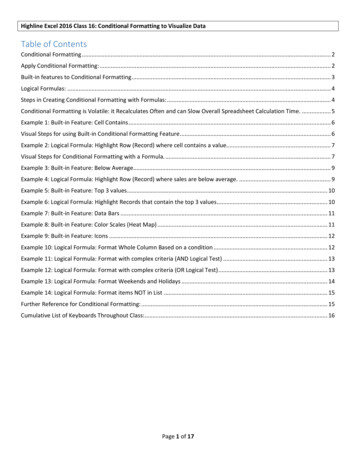
Example 3: Built-in Feature: Below AverageExample 4: Logical Formula: Highlight Row (Record) where sales are below average.Note: AVERAGE function had to calculate in every cell! This can slow down calculation in spreadsheet if:1. Ranges are large.2. There are many formulas.3. There are many different types of conditional formatting.Page 9 of 17
Example 5: Built-in Feature: Top 3 valuesExample 6: Logical Formula: Highlight Records that contain the top 3 valuesNote: LARGE function does NOT have to calculate in every cell in the Conditional Formatting range. Advantage to using a helper cell to calculate sub-calculations is that when the spreadsheet recalculates, only one cell has to calculate the LARGE value.Page 10 of 17
Example 7: Built-in Feature: Data Bars1) Data Bars creates an “In-Cell Bar Chart”. Max Longest Bar. Min Shortest Bar.2) Example:Example 8: Built-in Feature: Color Scales (Heat Map)1) Color Scale Ranks number by color.2) 3 colors: Red bottom 1/3 of values, Darkest Red Min. White middle 1/3 of values, White Mid-point (Median). Blue top 1/3 values, Darkest Blue Max.3) Example:Page 11 of 17
Example 9: Built-in Feature: Icons1) Icons can divide numbers into 3, groups (Top, middle, bottom)2) SIGN function delivers: Delivers -1 when number is negative. Delivers 0 when number is zero. Delivers 1 when number is positive.3) Example:Example 10: Logical Formula: Format Whole Column Based on a conditionPage 12 of 17
Example 11: Logical Formula: Format with complex criteria (AND Logical Test)1) AND Logical Test with AND function:Example 12: Logical Formula: Format with complex criteria (OR Logical Test)1) OR Logical Test with MATCH function (Is Item in List?):Page 13 of 17
Example 13: Logical Formula: Format Weekends and Holidays1) NETWORKDAYS.INTL function counts working days: NETWORKDAYS.INTL(start date , end date , weekend , holidays) weekend argument drop-down list: Normally it will count the number of weekdays between a start and end date. But if you give it the same start and end date, the function can only deliver either a one (1), it isa weekday, or zero (0), it is a weekend or holiday.2) Example:Page 14 of 17
Example 14: Logical Formula: Format items NOT in ListFurther Reference for Conditional Formatting:1) Highline Excel 2013 Class Video 40: Conditional Formatting Basic To Advanced 50 Exampleshttps://www.youtube.com/watch?v GRfe4bHsjhI2) Gantt Charts in Excel Playlist of Videoshttps://www.youtube.com/playlist?list PLrRPvpgDmw0mgjYXj7j9r2N9ObRXY45tnPage 15 of 17
Cumulative List of Keyboards Throughout Class:1) Esc Key:i. Closes Backstage View (like Print Preview).ii. Closes most dialog boxes.iii. If you are in Edit mode in a Cell, Esc will revert back to what you had in the cell before you put the Cell inEdit mode.2) F2 Key Puts formula in Edit Mode and shows the rainbow colored Range Finder.3) SUM Function: Alt 4) Ctrl Shift Arrow Highlight column (Current Region).5) Ctrl Backspace Jumps back to Active Cell6) Ctrl Z Undo.7) Ctrl Y Undo the Undo.8) Ctrl C Copy.9) Ctrl X Cut.10) Ctrl V Paste.11) Ctrl PageDown expose next sheet to right.12) Ctrl PageUp expose next sheet to left.13) Ctrl 1 Format Cells dialog box, or in a chart it opens Format Chart Element Task Pane.14) Ctrl Arrow: jumps to the bottom of the "Current Region", which means it jumps to the last cell that has data,right before the first empty cell.15) Ctrl Home Go to Cell A1.16) Ctrl End Go to last cell used.17) Alt keyboards are keys that you hit in succession. Alt keyboards are keyboards you can teach yourself by hittingthe Alt key and looking at the screen tips.i. Create PivotTable dialog box: Alt, N, Vii. Page Setup dialog box: Alt, P, S, Piii. Keyboard to open Sort dialog box: Alt, D, S18) ENTER When you are in Edit Mode in a Cell, it will put thing in cell and move selected cell DOWN.19) CTRL ENTER When you are in Edit Mode in a Cell, it will put thing in cell and keep cell selected.20) TAB When you are in Edit Mode in a Cell, it will put thing in cell and move selected cell RIGHT.21) SHIFT ENTER When you are in Edit Mode in a Cell, it will put thing in cell and move selected cell UP.22) SHIFT TAB When you are in Edit Mode in a Cell, it will put thing in cell and move selected cell LEFT.23) Ctrl T Create Excel Table (with dynamic ranges) from a Proper Data Set.i. Keyboard to name Excel Table: Alt, J, T, Aii. Tab Enter Raw Data into an Excel Table.24) Ctrl Shift ( ) General Number Formatting Keyboard.25) Ctrl ; Keyboard for hardcoding today's date.26) Ctrl Shift ; Keyboard for hardcoding current time.27) Arrow Key If you are making a formula, Arrow key will “hunt” for Cell Reference.28) Ctrl B Bold the Font29) Ctrl * (on Number Pad) or Ctrl Shift 8 Highlight Current Table.30) Alt Enter Add Manual Line Break (Word Wrap)31) Ctrl P Print dialog Backstage View and Print Preview32) F4 Key If you are in Edit mode while making a formula AND your cursor is touching a particular Cell Reference,F4 key will toggle through the different Cell References:i. A1 Relativeii. A 1 Absolute or “Locked”Page 16 of 17
)50)51)52)53)54)55)56)iii. A 1 Mixed with Row Locked (Relative as you copy across the columns AND Locked as you copy downthe rows)iv. A1 Mixed with Column Locked (Relative as you copy down the rows AND Locked as you across thecolumns)Ctrl Shift 4 Apply Currency Number FormattingTab key When you are selecting a Function from the Function Drop-down list, you can select the function thatis highlighted in blue by using the Tab key.F9 Key To evaluate just a single part of formula while you are in edit mode, highlight part of formula and hitthe F9 key.i. If you are creating an Array Constant in your formula: Hit F9.ii. If you are evaluating the formula element just to see what that part of the formula looks like,REMEMBER: to Undo with Ctrl Z.Alt, E, A, A Clear All (Content and Formatting)Evaluate Formula One Step at a Time Keyboard: Alt, M, VKeyboard to open Sort dialog box: Alt, D, SCtrl Shift L Filter (or Alt, D, F, F) Toggle key for Filter Drop-down ArrowsCtrl N Open New FileF12 Save As (Change File Name, Location, File Type)Import Excel Table into Power Query Editor: Alt, A, P, TCtrl 1 (When Chart element in selected): Open Task Pane for Chart ElementF4 Key If you are in Edit mode while making a formula AND your cursor is touching a particular Cell Reference,F4 key will toggle through the different Cell References:i. A1 Relativeii. A 1 Absolute or “Locked”iii. A 1 Mixed with Row Locked (Relative as you copy across the columns AND Locked as you copy downthe rows)iv. A1 Mixed with Column Locked (Relative as you copy down the rows AND Locked as you across thecolumns)Keyboard to open Scenario Manager Alt, T, ECtrl Tab Toggle between Excel Workbook File WindowsCtrl Shift F3 Create Names From SelectionCtrl F3 open Name ManagerF3 Paste Name or List of NamesAlt F4 Close Active WindowWindow Key Up Arrow Maximize Active WindowCtrl Shift Enter Keystroke to enter Array Formulas that: 1) have a function argument that requires it, or 2)whether or not you are entering the Resultant Array into multiple cells simultaneously.Ctrl / Highlight current ArrayData Validation Dialog Box: Alt, D, LF11 Create Chart on a new sheetAlt F11 Create Chart on currently selected sheet.New In This Video:57)58)59)60)New Format Rule dialog box: Alt, H, L, NDelete conditional Formatting Rule: Alt, O, D, DManage Rule dialog box keyboard: Alt, O, D“Format values where this formula is true”: Alt, H, L, N, PageDown, TabPage 17 of 17
Scrolling up or down causes Conditional Formatting to recalculate. 2) Conditional Formatting is recalculated when actions occur such as: Entering a formula. Inserting a column. Recalculating with the F9 key. 3) Conditional Formatting created with Logical Formulas slows down calculation in two ways: 1.