Transcription
EOSC 473/573Bamfield Exercise SummaryFebruary 18th to 20th, 2013Crew Members: Duckham, Carolyn; Volikhovska, Nataliya; Vora, Dhavan; Wang, Chuning.Work Distribution:Carolyn – Biology (Day 1) methods and resultsNataliya – Chemistry (Day 2) D.O. methods and results, Physics (Day 3) methods, andcompilationDhavan – Chemistry (Day 2) methods and resultsChuning – Physics (Day 3) results
Synopsis:Students enrolled in UBC’s Oceanographic Methods course participated in a week long field tripat Bamfield Marine Sciences Centre, February 17-23, 2013. Located on the west coast of VancouverIsland, this research facility gives students an opportunity to gain hands-on field and laboratory skills inbiological, chemical and physical sampling of the marine environment. The data report presented hereoutlines the objectives, methods, and data analyses undertaken on each of the themed days (Biology,Chemistry, and Physics) by the crew consisting of Nataliya, Dhavan, Chuning and Carolyn.Day 1: Biological SamplingIntroduction:On February 18th, the crew set out to sample planktonic communities at various distances from thecoastline in order to observe differences in species composition and abundance. The primary objectivewas to estimate phytoplankton and zooplankton carbon equivalents at various locations, but site selectionwas also driven by Nataliya’s and Dhavan’s research project looking at the spatial distribution of CDOM(chromophoric dissolved organic matter) from the coastline. CDOM plays a significant role in inhibitinglight penetration (therefore impacting photosynthesis), and is also known to significantly diminish beyondone nautical mile from the coastline (Foden et al., 2008). Being surrounded by coastline and limited bytime, our longest distance from the coastline was 0.63 nautical miles, hence differences in CDOM levelswere probably very small between sites, yet the crew hypothesized that phytoplankton abundance wouldbe higher at further distances from the coastline due to a possible reduction of CDOM (not measured).Methods:All sampling took place from 8:30am to 12:30 pm on Feb 18th onboard the Bamfield Twin Skiff,operated by Phil Lavoie. Personnel on board included Dr. Maite Maldonado, Chris Payne (sea-goingtechnician), and the crew of students (Nataliya, Dhavan, Chuning and Carolyn). A summary table of theday’s sampling details, weather conditions, and general results can be found in Table 1. A GPS was usedto locate our coordinates while on site, calibrated to NAD 83.Three sites were sampled: Site 1 in the Bamfield Inlet, Site 2 in the Trevor Channel, and Site 3 atthe mouth of the Bamfield Inlet (Figure 1). For Site 1, light intensity was measured at depth using aSecchi Disk and a light meter. After determining the depth at Site 1 using a depth sounder (32 m), thecrew conducted a vertical phytoplankton tow using a 50 µm mesh net from a 23 m depth. Using thewinch, the net was towed towards the surface at approximately 0.70 m/sec. Phytoplankton were collectedin the cod end of the net, rinsed with seawater, and collected into a pre-rinsed, labeled glass jar.Zooplankon was sampled at Site 1 using a 250 µm mesh net attached with a flow meter. An oblique towwas conducted at a depth of 17 m over a distance of 150 m. The tow depth was calculated using themathematical relationship adjacent cosΘ x hypotenuse, where Θ is the known angle of the rope beingdragged from the boat’s movement, the hypotenuse is the known length of the rope deployed from theboat, and by solving for “adjacent”, we would find our tow depth. The distance of the tow was calculatedusing the boats average speed (1.5 km/hr or 0.42 m/sec) multiplied by the duration of the tow (0.1 hr or360 sec). The net was not choked at depth, therefore upon completion of the tow, the net continuedvertically sampling zooplankton as it was retrieved to the surface at a speed of 0.70 m/sec using the winch.As the zooplankton net was pulled out of the sea, it was rinsed using a water pump to move allzooplankton down into the cod end. The cod end was then rinsed with seawater and the sample collectedin pre-rinsed, labeled glass jars. The filtration efficiency was calculated using the counts/sec, thenconverting them to water velocity by using the linear relationship on pg 6 in the flowmeter manual.2
For Site 2, very similar sampling activities took place as Site 1, except that zooplankton wassampled using a vertical tow from a 90 m depth, and phytoplankton was sampled from a 45 m depth. Dueto time constraints, only zooplankton was sampled at Site 3, in the mouth of Bamfield Inlet. Out ofinterest, two vertical tows for zooplankton were undertaken from a 40 m depth, with one tow using the125 µm mesh net and the other tow using the 250 µm mesh net, allowing for comparisons in zooplanktonabundance between net sizes. Unfortunately, two errors occurred with the sampling of the 125 µm meshtow: the cod end latch was not properly secured during the tow, and an accidental spill in the laboratorycaused the loss of the sample.Phytoplankton and zooplankton abundance and species composition were analyzed in thelaboratory in the afternoon on Feb 18th. Samples were not poisoned upon collection, and thereforeplanktonic organisms were free to feed on each other. Before samples were analyzed, the compoundmicroscope ocular scale was calibrated with a stage micrometer, and the field of view determined for the10x magnification. To determine phytoplankton abundance, a Sedgewick Rafter Counting Cell was used.To do this, a 1 ml aliquot of the well-mixed sample was placed into the Sedgewick Rafter, and the numberof phytoplankton were counted in randomly selected 1 µL square divisions of the counting cell, so that anaverage cells/µL could be calculated. For both sites, two 1 mL aliquots were analyzed for abundance (n 2). Using the density determined from the Sedgewick rafter, the abundance of phytoplankton in a cubicmeter volume of seawater (cells/m3) could be estimated for each site, by knowing the volume of thesample, and the total volume the phytoplankton net filtered through. A similar methodology was appliedto determine zooplankton abundance in a known volume of filtered seawater, except a counting tray witha 25 mL aliquot was used.In order to calculate the carbon equivalent of phytoplankton at each site many assumptions weremade. First, phytoplankton were identified (genus level) and sized only for Site 1, with the assumptionthat Site 2 had similar composition and size of organisms. Second, the volume of each phytoplankton cellwas assumed to be spherical, overestimating the cell volumes for some phytoplankton species such asCeratium tripos, which were measured along its longest axis. Third, species diversity was assumed to beevenly comprised as the length measures were averaged from the multiple species measured. To calculatethe carbon equivalents the formula given for phytoplankton (for diatoms) from The Manual of Chemicaland Biological Methods for Seawater Analysis was used (Parsons et al., 1984).Many assumptions were also used to estimate the zooplankton carbon equivalent. For example, itwas assumed that zooplankton had on average a cylinder shape of 1 mm length by 0.6 mm diameter,giving us a total volume of 0.28 mm3 for each zooplankton counted, or 0.00028 mL. In addition, the wetweight of zooplankton was assumed to be 1 gram for each ml, with a dry weight of 10% the total wetweight, therefore 0.000028 g per zooplankton. To calculate the carbon equivalents the formula given forzooplankton (mixed samples) from The Manual of Chemical and Biological Methods for SeawaterAnalysis was used (Parsons et al., 1984).Results and Discussion:i. Light IntensityLight attenuation graphs at Site 1 (Bamfield Inlet) and Site 2 (Trevor Channel) can be found inFigure 2. Reference lines on the figures represent secchi disk depth and calculated compensation depthfor each site. The compensation depth was calculated by determining the light extinction coefficient (k)for each site using equation Ih Io*e-kh (Site 1: k 0.16, Site 2: k 0.11), and by the assumption that thecompensation point was the same as the compensation irradiance for diatoms (7 µE/m2/sec). Though the3
secchi disk depth is deeper at Site 1 (14.45 m) versus Site 2 (13.38 m), it is evident that light ispenetrating slightly deeper at Site 2 than at Site 1, as the compensation depth is 7.79 m deeper, and thelight extinction coefficient is lower (Figure 2). The light meter is a more reliable source of data than thesecchi disk, which is more prone to human error. Light penetration into the water column was notsubstantially different between sites, but the deeper penetration at Site 2 (further away from the coast)may relate to lower CDOM levels expected at further distances away from land. However, the timedifference between light sampling was approximately 2 hrs, so it is possible that daylight was stronger atthe time of sampling at Site 2 versus Site 1, explaining the slight differences observed. Yet, it isimportant to point out that light irradiance at the surface for Site 1 was 114 µE/m2/s, and therefore slightlyhigher than Site 2 with105 µE/m2/s, implying that the daylight was not stronger during the sampling atSite 2.ii. Phytoplankton Abundance, Composition and Carbon EquivalenceOverall, phytoplankton abundance was really low at each site, possibly due to the large mesh size(50 µm) of the phytoplankton net used to collect the sample (Personal Communication: Dr. Maldonado).Phytoplankton abundance in the Bamfield Inlet (Site 1) was slightly higher than in the Trevor Channel(Site 2), with an average 68,488 cells/m3 and 56,840 cells/m3, respectively (Figure 3). A relatively largestandard error is present for both sites for various reasons: only 2 samples were analyzed for each site,live zooplankton were interfering with counts by disturbing and/or consuming phytoplankton, and humanerror due to students being new to counting phytoplankton cells (Figure 3). Phytoplankton abundancewas expected to be higher in the Trevor Channel as it was theorized that CDOM would be lower at furtherdistances from the coastline, yet the opposite trend was observed. Explanations as to why phytoplanktonabundance was slightly higher in the inlet may relate to the composition of the seawater, for example,higher concentrations of suspended matter, nutrients, or iron in the inlet compared to the channel.Zooplankton density (see next section) was similar at both sites, so the higher consumption ofphytoplankton at Site 2 is not a reasonable explanation. In addition, light intensity was similar at depth forboth sites, which also does not provide an explanation for the slight differences in abundances.Diatoms dominated the phytoplankton composition analyzed for Site 1 (only), comprising 95% ofthe taxa counted. This included Thalassiosira spp. (48%), Thalassionema nitzschioides (31%),Coscinodiscus spp. (8%), Pseudo-nitzchia (6%) and Rhizosolenia spp (1%), and Melosira spp. (1%)(Figure 4). Also observed was dinoflagellate Ceratium spp. (4%) and silicoflagellate Dictyocha fibula(1%).Similar to phytoplankton abundance, the carbon biomass for Site 1 was slightly higher than Site 2,with 0.25 mg/m3 and 0.21 mg/m3, respectively (Figure 5). Variation around the mean was fairly high dueto the same reasons for variation in abundance (small sample size, zooplankton interference and humanerror). The carbon biomass estimates were lower than the diatom carbon biomass presented in Cassis et al(2011) for March 2005 in Deep Bay (on the east coast of Vancouver Island), which ranged from 0.60 to0.70 mg/m3 (same as the unit µg/L) for diatoms. The slightly lower values observed in our sampling maybe due to location (being more exposed on the west coast of Vancouver Island), but is more likely a resultof the low abundance collected from sampling with the 50 µm phytoplankton net. In general, there is 50grams of carbon for each gram of chlorophyll a. Averaged over the water column, we found chlorophyll ato have a concentration of 0.30 mg/m3 on Day 2 of our field sampling. Therefore, the carbon biomassshould have been closer to 15 mg/ m3.4
iii. Zooplankton Abundance and Carbon EquivalenceZooplankton density was similar between all three sites, ranging from 476 to 532 organisms/m3(Figure 6). Zooplankton density was highest in Site 1, and may correspond to the slightly higherphytoplankton density occurring in the inlet. The zooplankton carbon biomass was similar across allthree sites, with values ranging from 1.41 to 2.18 mg/m3 (Figure 7). Zooplankton carbon biomass wasone order of magnitude higher than the phytoplankton carbon biomass, which could be because of thezooplankton’s larger size, but at the same time phytoplankton was observed to be much denser. Fromcomparing with a study by Uye et al (1999), who found zooplankton carbon biomass averaging around3.79 to 13.6 mg/m3 in Ise Bay (Japan) in Feb 1995, it appears our assumptions to calculate the carbonequivalent underestimates the actual values.iv. Filtration efficiencyThe filtration efficiency of the zooplankton oblique tow at Site 1 was 86% of the theoreticalvolume filtered (not including the vertical sampling that occurred retrieving the net from depth to thesurface). Therefore, we met the standard for the filtration efficiency (85% or greater) to avoid errorsrelated to zooplankton avoidance or clogging of net.FIGURESFigure 1. Site Locations for Biological Sampling5
Site 1: Bamfield InletSite 2: Trevor Channel2Light ( µ E/m /s)2Light ( µ E/m /s)020406080100012010102020Depth (m)Depth (m)2040608010012000304030405050Light MeterSecchi Disk (14.45m)Light MeterCompensation Depth (16.95m)Secchi Disk (13.38m)Compensation Depth (24.74m)Figure 2. Light attenuation at each site, including Secchi disk depth and compensation depthPhytoplankton Abundance(Average SE) (n 2 for each site)Abundance (cells/m 3)100,00080,00060,00040,00020,0000Site 1Site 2LocationFigure 3. Phytoplankton abundance at each site.6
Phytoplankton Taxa (Site 1)Total Cells 100Pseudo-nitzschia,6%Dictyocha fibula,1%Melosira spp., 1%Ceratium spp., 4%Thalassiosira spp.,48%Thalassionemanitzschioides, 31%Rhizosolenia spp.,Coscinodiscus1%spp., 8%Figure 4. Phytoplankton Genus Composition at Site 1Phytoplankton Carbon Equivalent(Average SE) (n 2 for each site)Carbon Biomass (mg/m 3)0.350.300.250.200.150.100.050.00Site 1Site 2LocationFigure 5. Estimated phytoplankton carbon biomass at each site.7
Zooplankton Abundance(n 1 for each site)Density (organims/m3)6005004003002001000Site 1Site 2Site 3LocationFigure 6. Zooplankton density at each site.Zooplankton Carbon Equivalence(n 1 for each site)Carbon Biomas (mg/m 3)2.52.01.51.00.50.0Site 1Site 2Site 3LocationFigure 7. Estimated zooplankton carbon biomass per site8
Table 1. Biology sampling details and general results.Zooplankton SamplingPhytoplanktonSamplingDetailsSite Name:Date:Vessel/OperatorSite 3: Mouth of BamfieldSite 2: Trevor ChannelInletFebruary 18, 2013Bamfield Skiff - Phil LavoieMaite Maldonado, Chris Payne, Phil Lavoie, Nataliya Volikhovska, Dhavan Vora,Chuning Wang & Carolyn Duckhamoooooo48.5001 N / 125.0083 W 48.5022 N / 125.0078 W48.5005 N / 125.0081 W9:00 to 10am10:30 to 11:30 am10:30 to 11:30 amOvercastOvercast/DrizzleOvercast/DrizzleCalm1 ft rollers1 ft icalNA2345NA5050NA0.700.70NASite 1: Bamfield InletPersonnel onboardLatitude/Longitude:Time:Weather:Sea State:Sounder Depth (m)Secchi Disk Depth (m)Compensation Depth (m)Tow TypeTow Depth (m)Net Size (µm)Tow Speed (m/s)3Volume Filtered (m )3Density (cells/m )Carbon Equivalent (mg3C/m )Tow TypeTow Depth (m)Tow Distance (m)Net Size (µm)Tow Speed (m/s)Filtration Efficiency (%)3Volume Filtered (m )3Density (organisms/m )Carbon Equivalent (mg3C/m tical40NA1250.60lost sample665324050418476lost samplelost sample2.181.791.41lost sampleREFERENCESFoden, J., Sivyer, D., Mills, D.K., and Devlin, M.J. 2008. Spatial and temporal distribution ofchromophoric dissolved organic matter (CDOM) fluorescence and its contribution to light attenuation inUK waterbodies. Estuarine, Coastal and Shelf Science. Vol 79 (4):707-717.Parsons, T.R., Maita, Y., and Lalli, C.M. 1984. A manual of chemical and biological methods forseawater analysis. Pergamon Press.Cassis, D., Lekhi, P., Pearce, C.M., Ebell, N., Orians, K., and Maldonado, M.T. 2011. The role ofphytoplankton in the modulation of dissolved and oyster cadmium concentrations in Deep Bay, BritishColumbia, Canada. Science of the Total Environment, 409: 4415 – 4424.Uye, S., Nagano, N., and Shimazu, T. 1999. Abundance, Biomass, Production and Trophic Roles ofMicro- and Net-Zooplankton in Ise Bay, Central Japan, in Winter. Journal of Oceanography Vol. 56:. 389to 398.9
Day 2: ChemistryIntroduction:The objective for February 19th was to collect seawater samples at various depths for dissolved oxygen,nitrate, and chlorophyll-a analysis using Niskin bottles. Our crew selected sites where CTD data wascollected the day before (by Group A), in order to potentially compare chemistry results with the physicalmeasurements. Efforts were made to select deep sites in order to obtain depth profiles of dissolvedoxygen, nitrate, and chlorophyll-a concentrations at those respective sites. Two sites were picked – one inImperial Eagle Channel, another in Trevor Channel – in order to compare the two water masses. Table 1outlines the details of our excursion.Table 1: Logistics and sampling details for February 19, 2013 (Day 2 - Chemistry).DateFebruary 19, 2013Time08:30am to 12:30pmWeatherSunny throughoutVesselALTAPersonnelJohn Richards, Chris Payne, Anne StewartCrew (Group C)Carolyn Duckham, Nataliya Volikhovska, Dhavan Vora, Chuning WangNiskin bottlesFive 5L, four 2LSITE 1Imperial Eagle ChannelDepth100mSampling time9:30am(approx.)Latitude148 50.889' N1Longitude125 08.956' WWavesSampling depths0, 5, 10, 20, 30, 40, 50, 70, 90(metres)Sampling volumes:Dissolved Oxygen2,31 x 125mLChlorophyll-a4,52 x 500mL6Nitrate2 x 100mLSITE 2Trevor Channel190m11:00am48 53.800' N125 03.067' W2 ft. rollers0, 5, 10, 20, 30, 50, 100, 150, 1801 x 125 mL2 x 500mL2 x 100mLComments1GPS device calibrated to NAD 83.D.O. samples were immediately pickled with MnSO4 and NaOH NaI reagents (in preparation for theWinkler method).3For depths of 0m and 30m at both sites, a replicate was sampled (2 x 125mL), totaling to 11 x 125mLsamples per site.4Chl-a samples were collected in two 500mL dark bottles per depth, but were later mixed and used as one1000mL sample (i.e. no replicates).5Samples for chlorophyll-a determination were only collected from euphotic zone (0, 5, 10, 20, 30m depths),totaling to 5 x 1000mL samples at each site.6Only 20mL of sample was used per replicate for nitrate determination.210
Methods:In the field Seawater samples were collected from 9 depths at each site, with intervals pre-determined based onexpected activity of three analytes – dissolved oxygen (D.O.), chlorophyll-a (chl-a), and nitrate. Asmentioned in Table 1, chl-a samples were collected only from the euphotic zone, and depths for D.O. andnitrate samples were chosen in order to create profiles from the surface to the deepest point possible (inthe case of Site 2, a hypoxic zone). The bottles, along with the CTD, were lowered at each site using thewinch onboard the Alta with the help of Captain John Richards. Using a messenger system, the bottleswere shut close, and were brought back up and placed on a convenient rack system to commencesampling. The five 5L Niskin bottles were used to sample the euphotic zone in order to compensate forchl-a samples.D.O. samples were collected first to minimize contact time between samples and atmospheric gases, i.e.reduced error in the true dissolved oxygen concentration. Once collected, they were immediately pickledwith MnSO4 and NaOH NaI so as to precipitate the D.O. out of solution (as Mn(OH)2), allowing for its“storage” in an accurate manner – eliminating the effect of further contamination on the analysis. Tworeplicates were collected for 0m and 30m depths to increase accuracy. In total, eleven 125mL D.O.samples were collected at each site. Following D.O. sampling, two 500mL bottles were used to collectchl-a samples in order to later combine them and analyse five 1000mL samples at each site. Dark, opaquebottles were used to reduce the chance of photodegradation of chl-a and other pigments relevant to ouranalysis. Lastly, two 100mL containers were used to sample for nitrate determination, adding up to 18total replicates per site. Though the containers were not opaque, they were stored in the dark to minimizefurther production of nutrients via photosynthesis. All sampling containers were rinsed with theirrespective samples in order to reduce contamination by residual matter.In the lab Dissolved Oxygen: D.O. concentrations were measured using the Winkler method. Due to technicaldifficulties, the analysis was carried out 24 hours later than planned. The precipitate (orange hues indicatepresence of oxygen) would then be dissolved by adding 3M sulfuric acid and shaking it. The quantitativeanalysis was done by an automatic titrator (Metrohm) by titrating the resulting solution with sodiumthiosulfate (Na2S2O3). The computer would then display the amount of dissolved oxygen present, as wellas the amount of sodium thiosulfate used.Chlorophyll-a analysis: Chlorophyll-a biomass was determined using fluorometry. Two 500mL replicateswere combined to make one 1000mL sample per sampling depth under the assumption that there wouldbe a lack in phytoplankton at these sites. Each sample was filtered through a standard grade-F filter(GF/F) and the filter stored in 8.0mL of cold 90% acetone. In order to speed up the extraction process ofchlorophyll-a and other pigments, the samples were put into a sonicator for 20 minutes, then a centrifugefor 5 minutes. Next, using a pre-calibrated fluorometer, the florescence of the acetone solution wasmeasured (“pre-acid”). Another measurement was recorded (“post-acid”) after adding 3 drops of HCl intothe acetone solution. The acidification allows for the determination of a ratio between the chlorophyll-apigment and other phaeo-pigments by shifting the fluorescence peak of chlorophyll-a, thus letting uscalculate chlorophyll-a biomass.11
Nitrate determination: The hydrazine reduction method from Strickland and Parsons (modified by NariSim) was used to reduce the nitrate in our samples (20mL) to nitrite, which was then diazotized withsulphanilamide and coupled with N-(10naphthyl)-ethylen-diamine to form a pink-coloured azo dye. Theintensity (absorbance) of this dye was measured using a spectrophotometer at λ 543nm. 20mL of eachsample was pipetted into an amber bottle and placed in a 23 C water bath. All reagents, including thebuffering and reducing reagents, were added while in the water bath. Once they were sufficientlyincubated, they were transferred into a 10cm longitudinal cuvette (10x more accurate than a 1cm cuvette)to measure the absorbance at 543nm.Results, Discussion:Chlorophyll-aThe difference between the pre-acid and post-acid fluorescence measurement of the acetone samplerepresents the fluorescence of chlorophyll-a, as the acidification represents the peak shift of chl-a at thatexcitation wavelength of the fluorometer. This ratio multiplied by the volume of acetone solution (0.008L) and 1.917 (calibration constant of given fluorometer setting) gives us the values for chlorophyll-abiomass in mg/m3. As seen in Figures 1 and 2, there is a clear trend in chlorophyll-a biomass in theeuphotic zone at Site 1 and 2 respectively. Given the two different water masses, Site 1 in the ImperialEagle Channel seems to have a deeper layer on the surface that is relatively low in chlorophyll-a biomass( 10m), whereas biomass at Site 2 in the Trevor Channel only takes 5m to reach its peak. Similarly, thedepth at which biomass rapidly decreases after the peak is 15-20m for Site 1 and 10m for Site 2. Thissuggests that bulk of the primary production at Site 2 occurs closer to the surface than at Site 1. It isimportant to note that our sample size (n 5; without replicates) is not good enough to make an accurateassumption. Human error in the lab process could have also produced erroneous data.NitrateThe process of nitrate determination was carried out in the lab without creating a standard curve; therefore,we acquired the standard curve data from Group A in order to use it to interpret our data. This may havecaused irregular data. Raw absorbance data was collected for most samples; an anomaly in thespectrophotometer resulted in the loss of 8 of 36 data points, therefore those replicates were not averaged.The data that was recorded also had many irregularities due to the abnormal behavior of thespectrophotometer (later found to be due to light contamination). Regardless of the faulty data, a verygeneral increase in the nitrate concentration with increasing depth is observed (Figures 3 and 4). This canbe explained by the consumption and excretion of nutrients (“marine snow”) by zooplankton. It isinteresting to note the sharp increase in nitrate concentration in the hypoxic zone at Site 2 because of theabsence of living organisms that could potentially consume these nutrients. Nevertheless, making anydeductions off this data would be highly inaccurate.Dissolved OxygenD.O. concentrations were determined by using the Metrohm titrator, and the titration curves were plottedautomatically using the associated software. However, due to technical difficulties on Feb 19th, oursamples could not be titrated. And due to limited time on Feb 20th, only few samples were analysed.Figures 5 and 6 show D.O. profiles at both sites. Again, it is interesting to note the hypoxic conditions thatare observed at Site 2 below the depth of 130m, where D.O. levels reach as low as 1mL/L. A fewgeneral assumptions can be made by looking at the CTD data for the two sites: since Site 1 (Imperial) hascolder water, it can explain the higher amount of D.O., whereas Site 2 (Trevor) is a warmer water masswith potential water mixing as shown by the D.O. and salinity wedges, thus having disturbed D.O. layersdown the profile.12
FIGURESFigure 1: Chlorophyll-a biomass profile, Site 1.Figure 2: Chlorophyll-a biomass profile, Site 2.13
Figure 3: Nitrate profile, Site 1. No replicates for depths 0, 5, 40, 50 and 70m.Figure 4: Nitrate profile, Site 2. No replicates for depths10, 30, 180m.14
Figure 5: D.O. profile, Site 1.Figure 6: D.O. profile, Site 2.15
Day 3: PhysicsIntroduction:On Feb 20th, our crew has set out to acquire CTD data at high tide from a transect starting at theshallow end of the Grappler Inlet and ending in the middle of the Trevor Channel (Figure 1). We chosethe following track in order to capture the salinity, temperature, and dissolved oxygen gradients that resultfrom freshwater flowing into the shallow end of the Grappler Inlet, as well as the Grappler Inlet waterexiting and mixing into the Trevor Channel water mass.Methods:All sampling took place from 8:30am to 12:30 pm on Feb 20th onboard the Bamfield Twin Skiff,operated by Phil Lavoie. Personnel on board included Dr. Rich Pawlowicz and the crew of students(Nataliya, Dhavan, Chuning and Carolyn). Attached are the CTD logs with sampling details and weatherconditions. A GPS was used to locate our coordinates while on site, calibrated to NAD 83. Stations 1 to 4are located inside the Grappler Inlet; Station 5 is near the mouth of Grappler Inlet; Stations 6 to 9 arelocated inside Trevor Channel (Figure 1).At each of the 9 sites (14 samplings in total, with replicates at stations 8, 6, 5, 4, and 2),temperature, ITS-90 [deg C] and salinity [ppt] at surface and at the depth of 0.5m would be recorded bythe YSI. Then, the CTD would be deployed. In order to lower the CTD, a generator was used to power thewinch at the speed of roughly 1 m/s. The time of turning on the switch was recorded, the CTD waslowered to the surface, where the time was recorded again, and the CTD would then soak for exactly 2minutes. After 2 minutes, the CTD was lowered to the desired depth, the time at which it reached thebottom was recorded, and the CTD was raised up immediately afterwards. The last time to be recorded isthe turning off of the switch. The CTD recorded the following values: Pressure, Strain Gauge [db],Temperature, ITS-90 [deg C], Conductivity [mS/cm] as well as dissolved oxygen, SBE 43 [V]. Thesample rate was set to 1 scan every 0.5 seconds.Once in the lab, the data was downloaded into the bamfield13 hex directory, and the log files weremodified to include the exact time, latitude, longitude, depth, station name, and any comments we haverecorded. Data processing came next, using SBEDataProc. First, the data was converted from hex to rawunits specified above, and plotted in order to see if the data made sense. Then, the temperature,conductivity, and pressure sensors were adjusted to the right filters to give equal responses or to removequantization errors. Alignment was then done (T 0.5s, O2 7s) to correct for varying sensor speeds.Loop edit wasn’t necessary in this case due to fairly calm waters. Afterwards, practical salinity, PSS78[PSU] and oxygen saturation [ml/L] were derived. The data was then graphed again in order to find thecorrect scan number after the soak to use for binning, and binning (size of 1m) was performed to obtainevenly-spaced data.Results and Discussion:i. Topography:Along the track, water depth increases until it reaches 110 m (Trevor Channel, 3.9 km), thendecreases to 70 m at the end of the track. During the first 2.4 km of the track, the depth hasn’t changed toomuch (from 5 m to 20 m), then the seafloor drops quickly from 20 m to 110 m.ii. Temperat
10x magnification. To determine phytoplankton abundance, a Sedgewick Rafter Counting Cell was used. To do this, a 1 ml aliquot of the well-mixed sample was placed into the Sedgewick Rafter, and the number of phytoplankton were counted in randomly selected 1 µL square divisions of the counting cell, so that an average cells/µL could be calculated.