Transcription
Loop and Spin Foam Quantum Gravity:A Brief Guide for BeginnersH. Nicolai1 and K. Peeters212Max-Planck-Institut für Gravitationsphysik, Albert-Einstein-Institut,Am Mühlenberg 1, 14476 Golm, ut für Gravitationsphysik, Albert-Einstein-Institut,Am Mühlenberg 1, 14476 Golm, GermanyKasper.Peeters@aei.mpg.de1 Quantum Einstein GravityThe assumption that Einstein’s classical theory of gravity can be quantisednon-perturbatively is at the root of a wide variety of approaches to quantumgravity. The assumption constitutes the basis of several discrete methods [1],such as dynamical triangulations and Regge calculus, but it also implicitlyunderlies the older Euclidean path integral approach [2, 3] and the somewhatmore indirect arguments which suggest that there may exist a non-trivial fixedpoint of the renormalisation group [4–6]. Finally, it is the key assumptionwhich underlies loop and spin foam quantum gravity. Although the assumption is certainly far-reaching, there is to date no proof that Einstein gravitycannot be quantised non-perturbatively, either along the lines of one of theprograms listed above or perhaps in an entirely different way.In contrast to string theory, which posits that the Einstein–Hilbert actionis only an effective low-energy approximation to some other, more fundamental, underlying theory, loop and spin foam gravity takes Einstein’s theory infour space-time dimensions as the basic starting point, either with the conventional or with a (constrained) ‘BF-type’ formulation.1 These approachesare background independent in the sense that they do not presuppose the existence of a given background metric. In comparison to the older geometrodynamics approach (which is also formally background independent) they makeuse of many new conceptual and technical ingredients. A key role is playedby the reformulation of gravity in terms of connections and holonomies. A related feature is the use of spin networks in three (for canonical formulations)1In the remainder, we will often follow established (though perhaps misleading)custom and summarily refer to this framework of ideas simply as ‘Loop QuantumGravity’, or LQG for short.H. Nicolai and K. Peeters: Loop and Spin Foam Quantum Gravity: A Brief Guide forBeginners, Lect. Notes Phys. 721, 151–184 (2007)c Springer-Verlag Berlin Heidelberg 2007DOI 10.1007/978-3-540-71117-9 9
152H. Nicolai and K. Peetersand four (for spin foams) dimensions. These, in turn, require other mathematical ingredients, such as non-separable (‘polymer’) Hilbert spaces andrepresentations of operators which are not weakly continuous. Undoubtedly,novel concepts and ingredients such as these will be necessary in order tocircumvent the problems of perturbatively quantised gravity (that novel ingredients are necessary is, in any case, not just the point of view of LQG butalso of most other approaches to quantum gravity). Nevertheless, it is important not to lose track of the physical questions that one is trying to answer.Evidently, in view of our continuing ignorance about the ‘true theory’ ofquantum gravity, the best strategy is surely to explore all possible avenues.LQG, just like the older geometrodynamics approach [7], addresses several aspects of the problem that are currently outside the main focus of string theory,in particular the question of background independence and the quantisationof geometry. Whereas there is a rather direct link between (perturbative)string theory and classical space-time concepts, and string theory can therefore rely on familiar notions and concepts, such as the notion of a particleand the S-matrix, the task is harder for LQG, as it must face up right awayto the question of what an observable quantity is in the absence of a propersemi-classical space-time with fixed asymptotics.The present text, which is based in part on the companion review [8], isintended as a brief introductory and critical survey of loop and spin foamquantum gravity,2 with special attention to some of the questions that arefrequently asked by non-experts, but not always adequately emphasised (forour taste, at least) in the pertinent literature. For the canonical formulationof LQG, these concern in particular the definition and implementation ofthe Hamiltonian (scalar) constraint and its lack of uniqueness. An importantquestion (which we will not even touch on here) concerns the consistent incorporation of matter couplings, and especially the question as to whether theconsistent quantisation of gravity imposes any kind of restrictions on them. Establishing the existence of a semi-classical limit, in which classical space-timeand the Einstein field equations are supposed to emerge, is widely regardedas the main open problem of the LQG approach. This is also a prerequisitefor understanding the ultimate fate of the non-renormalisable UV divergencesthat arise in the conventional perturbative treatment. Finally, in any canonical approach there is the question whether one has succeeded in achieving (aquantum version of) full space-time covariance, rather than merely covarianceunder diffeomorphisms of the three-dimensional slices. In [8] we have argued(against a widely held view in the LQG community) that for this, it is notenough to check the closure of two Hamiltonian constraints on diffeomorphisminvariant states, but that it is rather the off-shell closure of the constraint algebra that should be made the crucial requirement in establishing quantumspace-time covariance.2Whereas [8] is focused on the ‘orthodox’ approach to loop quantum gravity, towit the Hamiltonian framework.
Loop and Spin Foam Quantum Gravity: A Brief Guide for Beginners153Many of these questions have counterparts in the spin foam approach,which can be viewed as a ‘space-time covariant version’ of LQG, and at thesame time as a modern variant of earlier attempts to define a discretised pathintegral in quantum gravity. For instance, the existence of a semi-classical limitis related to the question whether the Einstein–Hilbert action can be shown toemerge in the infrared (long distance) limit, as is the case in (2 1) gravity inthe Ponzano–Regge formulation, cf. (38). Regarding the non-renormalisableUV divergences of perturbative quantum gravity, many spin foam practitioners seem to hold the view that there is no need to worry about short distancesingularities and the like because the divergences are simply ‘not there’ inspin foam models, due to the existence of an intrinsic cutoff at the Planckscale. However, the same statement applies to any regulated quantum fieldtheory (such as lattice gauge theory) before the regulator is removed, and onthe basis of this more traditional understanding, one would therefore expectthe ‘correct’ theory to require some kind of refinement (continuum) limit,3or a sum ‘over all spin foams’ (corresponding to the ‘sum over all metrics’in a formal path integral). If one accepts this point of view, a key questionis whether it is possible to obtain results which do not depend on the specific way in which the discretisation and the continuum limit are performed(this is also a main question in other discrete approaches which work withreparametrisation invariant quantities, such as in Regge calculus). On theother hand, the very need to take such a limit is often called into questionby LQG proponents, who claim that the discrete (regulated) model correctlydescribes physics at the Planck scale. However, it is then difficult to see (and,for gravity in (3 1) dimensions, has not been demonstrated all the way in asingle example) how a classical theory with all the requisite properties, andin particular full space-time covariance, can emerge at large distances. Furthermore, without considering such limits, and in the absence of some otherunifying principle, one may well remain stuck with a multitude of possiblemodels, whose lack of uniqueness simply mirrors the lack of uniqueness thatcomes with the need to fix infinitely many coupling parameters in the conventional perturbative approach to quantum gravity.Obviously, a brief introductory text such as this cannot do justice to thenumerous recent developments in a very active field of current research. Forthis reason, we would like to conclude this introduction by referring readersto several ‘inside’ reviews for recent advances and alternative points of view,namely [9–11] for the canonical formulation, [12–14] for spin foams, and [15]for both. A very similar point of view to ours has been put forward in [16, 17].4Readers are also invited to have a look at [18] for an update on the very latestdevelopments in the subject.34Unless quantum gravity is ultimately a topological theory, in which case thesequence of refinements becomes stationary. Such speculations have also beenentertained in the context of string and M theory.However, [16, 17] only addresses the so-called ‘m-ambiguity’, whereas we willargue that there are infinitely many other parameters which a microscopic theoryof quantum gravity must fix.
154H. Nicolai and K. Peeters2 The Kinematical Hilbert Space of LQGThere is a general expectation (not only in the LQG community) that at thevery shortest distances, the smooth geometry of Einstein’s theory will be replaced by some quantum space or space-time, and hence the continuum willbe replaced by some ‘discretuum’. Canonical LQG does not do away withconventional spacetime concepts entirely, in that it still relies on a spatialcontinuum Σ as its ‘substrate’, on which holonomies and spin networks live(or ‘float’) – of course, with the idea of eventually ‘forgetting about it’ byconsidering abstract spin networks and only the combinatorial relations between them. On this substrate, it takes as the classical phase space variablesthe holonomies of the Ashtekar connection, a.(1)he [A] P exp Aam τa dxm , with Aam : 21 !abc ωmbc γ KmeHere, τa are the standard generators of SU(2) (Pauli matrices), but one canalso replace the basic representation by a representation of arbitrary spin,denoted by ρj (he [A]). The Ashtekar connection A is thus a particular linaear combination of the spin connection ωmbc and the extrinsic curvature Kmwhich appear in a standard (3 1) decomposition. The parameter γ is the socalled ‘Barbero-Immirzi parameter’. The variable conjugate to the Ashtekarconnection turns out to be the inverse densitised dreibein Ẽa m : e ea m . Using this conjugate variable, one can find the objects which are conjugate tothe holonomies. These are given by integrals of the associated two-form overtwo-dimensional surfaces S embedded in Σ, !mnp Ẽam f a dxn dxp ,(2)FS [Ẽ, f ] : Swhere f a (x) is a test function. This flux vector is indeed conjugate to theholonomy in the sense described in Fig. 1: if the edge associated to the holonomy intersects the surface associated to the flux, the Poisson bracket betweenthe two is non-zero,# (he [A])αβ , FS [Ẽ, f ] γ fa (P ) he1 [A] τ a he2 [A] αβ ,(3)where e e1 e2 and the sign depends on the relative orientation of the edgeand the two-surface. This Poisson structure is the one which gets promotedto a commutator algebra in the quantum theory.Instead of building a Hilbert space as the space of functions over configurations of the Ashtekar connection, i.e. instead of constructing wave-functionalsΨ [Am (x)], LQG uses a Hilbert space of wave functionals which “probe” thegeometry only on one-dimensional submanifolds, the so-called spin networks.The latter are (not necessarily connected) graphs Γ embedded in Σ consistingof finitely many edges (links). The wave functionals are functionals over the
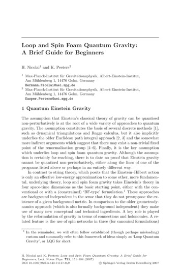
Loop and Spin Foam Quantum Gravity: A Brief Guide for Beginners155e2e1Fig. 1. LQG employs holonomies and fluxes as elementary conjugate variables.When the edge of the holonomy and the two-surface element of the flux intersect, thecanonical Poisson bracket of the associated operators is non-vanishing, and insertsa τ -matrix at the point of intersection, cf. (3)space of holonomies. In order to make them C-valued, the SU(2) indices of theholonomies have to be contracted using invariant tensors (i.e. Clebsch–Gordancoefficients). The wave function associated to the spin network in Fig. 2 is,for instance, given by%&&%ρj2 (he2 [A])Ψ [fig.2] ρj1 (he1 [A])α1 β1%α2 β2& ρj3 (he3 [A])α3 β3Cβj11jβ22jβ33 . . . ,(4)where dots represent the remainder of the graph. The spin labels j1 , . . . mustobey the standard rules for the vector addition of angular momenta, butotherwise can be chosen arbitrarily. The spin network wave functions Ψ arethus labelled by Γ (the spin network graph), by the spins {j} attached to theedges, and the intertwiners {C} associated to the vertices.At this point, we have merely defined a space of wave functions in termsof rather unusual variables, and it now remains to define a proper Hilbertspace structure on them. The discrete kinematical structure which LQG imposes does, accordingly, not come from the description in terms of holonomiesand fluxes. After all, this very language can also be used to describe ordinary Yang–Mills theory. The discrete structure which LQG imposes is alsoentirely different from the discreteness of a lattice or naive discretisation ofspace (i.e. of a finite or countable set). Namely, it arises by ‘polymerising’ thecontinuum via an unusual scalar product . For any two spin network states,one defines this scalar product to be ('ΨΓ,{j},{C} ΨΓ ,{j },{C } if Γ Γ , 0(5) dhei ψ̄Γ,{j},{C} ψΓ ,{j },{C } if Γ Γ , ei Γ
156H. Nicolai and K. PeetersΣυ4e6e1e4υ1e3υ3e2υ2e5Fig. 2. A simple spin network, embedded in the spatial hypersurface Σ. The hypersurface is only present in order to provide coordinates which label the positions ofthe vertices and edges. Spin network wave functions only probe the geometry alongthe one-dimensional edges and are insensitive to the geometry elsewhere on Σ where the integrals dhe are to be performed with the SU(2) Haar measure.The spin network wave functions ψ depend on the Ashtekar connection onlythrough the holonomies. The kinematical Hilbert space Hkin is then defined asthe completion of the space of spin network wave functions w.r.t. this scalarproduct (5). The topology induced by the latter is similar to the discretetopology (‘pulverisation’) of the real line with countable unions of points asthe open sets. Because the only notion of ‘closeness’ between two points inthis topology is whether or not they are coincident, whence any function iscontinuous in this topology, this raises the question as to how one can recoverconventional notions of continuity in this scheme.The very special choice of the scalar product (5) leads to representations ofoperators which need not be weakly continuous: this means that expectationvalues of operators depending on some parameter do not vary continuously asthese parameters are varied. Consequently, the Hilbert space does not admita countable basis, hence is non-separable, because the set of all spin networkgraphs in Σ is uncountable, and non-coincident spin networks are orthogonalw.r.t. (5). Therefore, any operation (such as a diffeomorphism) which movesaround graphs continuously corresponds to an uncountable sequence of mutually orthogonal states in Hkin . That is, no matter how ‘small’ the deformationof the graph in Σ, the associated elements of Hkin always remain a finitedistance apart, and consequently, the continuous motion in ‘real space’ getsmapped to a highly discontinuous one in Hkin . Although unusual, and perhaps counter-intuitive, as they are, these properties constitute a cornerstonefor the hopes that LQG can overcome the seemingly unsurmountable problems of conventional geometrodynamics: if the representations used in LQGwere equivalent to the ones of geometrodynamics, there would be no reasonto expect LQG not to end up in the same quandary.
Loop and Spin Foam Quantum Gravity: A Brief Guide for Beginners157Because the space of quantum states used in LQG is very different fromthe one used in Fock space quantisation, it becomes non-trivial to see howsemi-classical ‘coherent’ states can be constructed, and how a smooth classical space-time might emerge. In simple toy examples, such as the harmonicoscillator, it has been shown that the LQG Hilbert space indeed admits states(complicated linear superpositions) whose properties are close to those of theusual Fock space coherent states [19]. In full (3 1)-dimensional LQG, theclassical limit is, however, far from understood (so far only kinematical coherent states are known [20–25], i.e. states which do not satisfy the quantumconstraints). In particular, it is not known how to describe or approximateclassical space-times in this framework that ‘look’ like, say, Minkowski space,or how to properly derive the classical Einstein equations and their quantum corrections. A proper understanding of the semi-classical limit is alsoindispensable to clarify the connection (or lack thereof) between conventionalperturbation theory in terms of Feynman diagrams and the non-perturbativequantisation proposed by LQG.However, the truly relevant question here concerns the structure (and definition!) of physical space and time. This, and not the kinematical ‘discretuum’on which holonomies and spin networks ‘float’, is the arena where one shouldtry to recover familiar and well-established concepts like the Wilsonian renormalisation group, with its continuous ‘flows’. Because the measurement oflengths and distances ultimately requires an operational definition in termsof appropriate matter fields and states obeying the physical state constraints,‘dynamical’ discreteness is expected to manifest itself in the spectra of the relevant physical observables. Therefore, let us now turn to a discussion of thespectra of three important operators and to the discussion of physical states.3 Area, Volume, and the HamiltonianIn the current setup of LQG, an important role is played by two relativelysimple operators: the ‘area operator’ measuring the area of a two-dimensionalsurface S Σ and the ‘volume operator’ measuring the volume of a threedimensional subset V Σ. The latter enters the definition of the Hamiltonianconstraint in an essential way. Nevertheless, it must be emphasised that thearea and volume operators are not observables in the Dirac sense, as they donot commute with the Hamiltonian. To construct physical operators corresponding to area and volume is more difficult and would require the inclusionof matter (in the form of ‘measuring rod fields’).The area operator is most easily expressed as dF a · dF a , with dFa : !mnp Ẽam dxn dxp(6)AS [g] S(the area element is here expressed in terms of the new ‘flux variables’ Ẽam , butis equal to the standard expression dFa : !abc em b en c dxm dxn ). The next
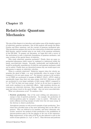
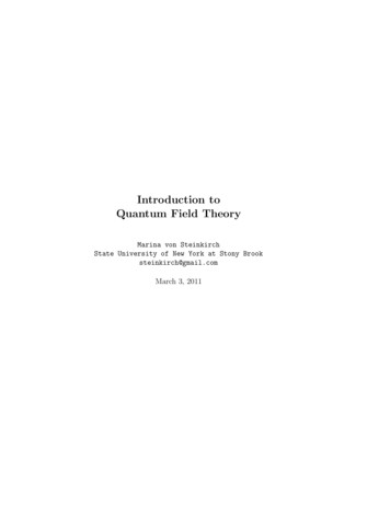
158H. Nicolai and K. Peetersstep is to rewrite this area element in terms of the spin network variables,in particular the momentum Ẽa m conjugate to the Ashtekar connection. Inorder to do so, we subdivide the surface into infinitesimally small surfaces SIas in Fig. 3. Next, one approximates the area by a Riemann sum (which, ofcourse, converges for well-behaved surfaces S), using dF a · dF a FSaI [Ẽ] FSaI [Ẽ] .(7)SIThis turns the operator into the expressionN aAS [Ẽm] limFSaI [Ẽ] FSaI [Ẽ] .N (8)I 1If one applies the operator (8) to a wave function associated with a fixed graphΓ and refines it in such a way that each elementary surface SI is pierced byonly one edge of the network, one obtains, making use of (3) twice,ÂS Ψ 8πlp2 γ#edges jp (jp 1) Ψ .(9)p 1These spin network states are thus eigenstates of the area operator. The situation becomes considerably more complicated for wave functions which containa spin network vertex which lies in the surface S; in this case the area operatordoes not necessarily act diagonally anymore (see Fig. 4). Expression (9) liesat the core of the statement that areas are quantised in LQG.The construction of the volume operator follows similar logic, although itis substantially more involved. One starts with the classical expression for thevolume of a three-dimensional region Ω Σ,. 1 3mnpabc (10)Ẽm Ẽn Ẽp .d x !abc !V (Ω) 3!ΩFig. 3. The computation of the spectrum of the area operator involves the divisionof the surface into cells, such that at most one edge of the spin network intersectseach given cell
Loop and Spin Foam Quantum Gravity: A Brief Guide for Beginners112343215912344Fig. 4. The action of the area operator on a node with intertwiner Cαj11jα22kβ Cαj33jα44kβ .Whether or not this action is diagonal depends on the orientation of the surfaceassociated to the area operator. In the figure on the (left), the location of theedges with respect to the surface is such that the invariance of the Clebsch–Gordancoefficients can be used to evaluate the action of the area operator. The result canbe written in terms of a ‘virtual’ edge. In the figure on the (right), however, this isnot the case, a recoupling relation is needed, and the spin network state is not aneigenstate of the corresponding area operatorJust as with the area operator, one partitions Ω into small cells Ω I ΩI ,so that the integral can be replaced with a Riemann sum. In order to expressthe volume element in terms of the canonical quantities introduced before,one then again approximates the area elements dF a by the small but finitearea operators FSa [Ẽ], such that the volume is obtained as the limit of aRiemann sum. N 1 !abc F a1 [Ẽ] F b 2 [Ẽ] F c3 [Ẽ] .(11)V (Ω) lim SSSIIIN 3!I 1The main problem is now to choose appropriate surfaces S1,2,3 in each cell.This should be done in such a way that the r.h.s. of (11) reproduces the correctclassical value. For instance, one can choose a point inside each cube ΩI , thenconnect these points by lines and ‘fill in’ the faces. In each cell ΩI one thenhas three lines labelled by a 1, 2, 3; the surface SIa is then the one that istraversed by the a-th line. With this choice it can be shown that the result isinsensitive to small ‘wigglings’ of the surfaces, hence independent of the shapeof SIa , and the above expression converges to the desired result. See [26, 27]for some recent results on the spectrum of the volume operator.The key problem in canonical gravity is the definition and implementation of the Hamiltonian (scalar) constraint operator, and the verification thatthis operator possesses all the requisite properties. The latter include (quantum) space-time covariance as well as the existence of a proper semi-classicallimit, in which the classical Einstein equations are supposed to emerge. It isthis operator which replaces the Hamiltonian evolution operator of ordinaryquantum mechanics, and encodes all the important dynamical informationof the theory (whereas the Gauss and diffeomorphism constraints are merely‘kinematical’). More specifically, together with the kinematical constraints,
160H. Nicolai and K. Peetersit defines the physical states of the theory, and thereby the physical Hilbertspace Hphys (which may be separable [28], even if Hkin is not).To motivate the form of the quantum Hamiltonian one starts with theclassical expression, written in loop variables. To this aim one rewrites theHamiltonian in terms of Ashtekar variables, with the result H[N ] &Ẽ m Ẽ n %1d3 x N a b !abc Fmnc (1 γ 2 )K[m a Kn] b .2Σdet Ẽ(12)For the special values γ i, the last term drops out, and the Hamiltonian simplifies considerably. This was indeed the value originally proposed byAshtekar, and it would also appear to be the natural one required by localLorentz invariance (as the Ashtekar variable is, in this case, just the pullbackof the four-dimensional spin connection). However, imaginary γ obviously implies that the phase space of general relativity in terms of these variableswould have to be complexified, such that the original phase space could berecovered only after imposing a reality constraint. In order to avoid the difficulties related to quantising this reality constraint, γ is now usually taken tobe real. With this choice, it becomes much more involved to rewrite (12) interms of loop and flux variables.4 Implementation of the ConstraintsIn canonical gravity, the simplest constraint is the Gauss constraint. In thesetting of LQG, it simply requires that the SU(2) representation indices entering a given vertex of a spin network enter in an SU(2) invariant manner. More complicated are the diffeomorphism and Hamiltonian constraint.In LQG these are implemented in two entirely different ways. Moreover, theimplementation of the Hamiltonian constraint is not completely independent,as its very definition relies on the existence of a subspace of diffeomorphisminvariant states.Let us start with the diffeomorphism constraint. Unlike in geometrodynamics, one cannot immediately write down formal states which are manifestly diffeomorphism invariant, because the spin network functions are notsupported on all of Σ, but only on one-dimensional links, which ‘move around’under the action of a diffeomorphism. A formally diffeomorphism invariantstate is obtained by ‘averaging’ over the diffeomorphism group, and morespecifically by considering the formal sum ΨΓ [A φ] .(13)η(Ψ )[A] : φ Diff(Σ Γ )Here Diff(Σ Γ ) is obtained by dividing out the diffeomorphisms leaving invariant the graph Γ . Although this is a continuous sum which might seem to
Loop and Spin Foam Quantum Gravity: A Brief Guide for Beginners161be ill-defined, it can be given a mathematically precise meaning because theunusual scalar product (5) ensures that the inner product between a state anda diffeomorphism-averaged state, φ ΨΓ ΨΓ ,(14) η(ΨΓ ) ΨΓ φ Diff(Σ Γ )consists at most of a finite number of terms. It is this fact which ensuresthat η(ΨΓ ) is indeed well defined as an element of the space dual to thespace of spin networks (which is dense in Hkin ). In other words, althoughη(Ψ ) is certainly outside of Hkin , it does make sense as a distribution. On thespace of diffeomorphism averaged spin network states (regarded as a subspaceof a distribution space) one can now again introduce a Hilbert space structure‘by dividing out’ spatial diffeomorphisms, namely η(Ψ ) η(Ψ ) : η(Ψ ) Ψ .(15)The completion by means of this scalar product defines the space Hdiff ; butnote that Hdiff is not a subspace of Hkin !As mentioned above, however, it is the Hamiltonian constraint which playsthe key role in canonical gravity, as it this operator which encodes the dynamics. Implementing this constraint on Hdiff or some other space is fraughtwith numerous choices and ambiguities, inherent in the construction of thequantum Hamiltonian as well as the extraordinary complexity of the resultingexpression for the constraint operator [29]. The number of ambiguities can bereduced by invoking independence of the spatial background [10], and indeed,without making such choices, one would not even obtain sensible expressions.In other words, the formalism is partly ‘on-shell’ in that the very existence ofthe (unregulated) Hamiltonian constraint operator depends very delicately onits ‘diffeomorphism covariance’, and the choice of a proper ‘habitat’, on whichit is supposed to act in a well-defined manner. A further source of ambiguities,which, for all we know, has not been considered in the literature so far, consists in possible -dependent ‘higher order’ modifications of the Hamiltonian,which might still be compatible with all consistency requirements of LQG.In order to write the constraint in terms of only holonomies and fluxes, onehas to eliminate the inverse square root Ẽ 1/2 in (12) as well as the extrinsiccurvature factors. This can be done through a number of tricks found byThiemann [30]. The vielbein determinant is eliminated using!mnp !abc Ẽ 1/2 Ẽb n Ẽc p 1 #Am a (x), V .4γ(16)where V V (Σ) is the total volume, cf. (10). The extrinsic curvature iseliminated by writing it as 1Km a (x) Am a (x) , K̄whereK̄ : d3 x Km a Ẽa m ,(17)γΣ
162H. Nicolai and K. Peetersand then eliminating the integrand of K̄ using 1 # Ẽa m Ẽb n abc ! Fmnc (x), VẼ 1 mnp #{Am a , V }Fnpa , V , 5/2 !4γK̄(x) γ 3/2(18)i.e. writing it as a nested Poisson bracket. Inserting these tricks into the Hamiltonian constraint, one replaces (12) with the expression %d3 x N !mnp Tr Fmn {Ap , V }H[N ] Σ&1 (1 γ 2 ){Am , K̄}{An , K̄}{Ap , V } ,2(19)with K̄ understood to be eliminated using (18). This expression, which nowcontains only the connection A and the volume V , is the starting point forthe construction of the quantum constraint operator.In order to quantise the classical Hamiltonian (19), one next elevates allclassical objects to quantum operators as described in the foregoing sections,and replaces the Poisson brackets in (19) by quantum commutators. The resulting regulated Hamiltonian then reduces to a sum over the vertices vα ofthe spin network with lapses N (vα )Ĥ[N, !] αN (vα ) !mnp 1 / 0hp , V̂ Tr h Pmn ( ) h 1 Pmn ( ) hp 2 112 (1 γ )hm/hm , K̄0h 1n/hn , K̄0h 1p 0/,hp , V̂(20)where Pmn (!) is a small loop attached to the vertex vα that must eventually be shrunk to zero. In writing the above expression, we have furthermoreassumed a specific (but, at this point, not specially preferred) ordering of theoperators.Working out the action of (20) on a given spin network wave function israther non-trivial, and we are not aware of any concrete calculations in thisregard, other than for very simple special configurations (see, e.g., [31]); toget an idea of the complications, readers may have a look at a recent analysisof the volume operator and its spectrum in [32]. In particular, the availablecalculations focus almost exclusively on the action of the first term in (20),whereas the second term (consisting of multiply nested commutators, cf. (18))is usually not discussed in any detail. At any rate, this calculation involvesa number of choices in order to fix
H. Nicolai and K. Peeters:Loop and Spin Foam Quantum Gravity: A Brief Guide for Beginners, Lect. Notes Phys.721, 151-184 (2007) DOI 10.1007/978-3-540-71117-9 9 c Springer-Verlag Berlin Heidelberg 2007. . describes physics at the Planck scale. However, it is then difficult to see (and, for gravity in (3 1) dimensions, has not been .