Transcription
Quantum Error Correction CodesDong-Sheng WangApril 21, 2021Definition. A quantum code is usually defined by a linear encodingisometry V : Hl C H, and an error correction code is a triple(V, N , R), which requires the ability to fully recovery any state ψi Cby a recovery channel R after a prescribed noise channel N acting onthe code space C.KeywordsEncoding; linear codes; error correction; approximate codes; coding bounds;stabilizer codes; toric code; LDPC codes; fault tolerance; universality; threshold; error control; self correction.AbstractWe explain quantum codes and fault-tolerant quantum computing. In order to perform reliable quantum computing, wehave to use qubits encoded in error-correction codes. We first explain the basics of quantum codes, including encoding isometry,error correction and detection, code distance, encoding bounds,logical gates, recovery channel, etc. Then we introduce stabilizer codes and describe some examples. Next we explain howto use quantum error-correction codes for quantum computing,1
with a notable candidate: color code. Finally, we survey otherways of dealing with decoherence and some frontiers, and alsostories.11.1Minimal versionOpeningThe subject of quantum error correction (QEC) has been developed for two decades, just a little bit shorter than quantumcomputing itself. QEC is the most crucial part for quantumcomputing since it ensures the computation to be reliable, otherwise the output of a computing device is just crap. So everyquantum computer scientist has to understand QEC and theframework of fault-tolerant quantum computing.The very starting idea is encoding, which also lies at the heartof all classical communication, computing, cryptography, andrelevant fields. The encoding can be used to protect againstnoise or enemy. Encoding refers to the process to use redundancy to enhance the robustness of information against noises(errors). For instance, we can encode 0 as a string of 0s and 1 asa string of 1s, so that flips of a few bits do not affect the information we encode. Information processing occurs in an encodedway: first encode, then do operations you want, then decode,and finally readout the results you need. Furthermore, encodingalso occurs in natural physical systems: macroscopic observableis encoded in microscopic details of statistical systems, the interior bulk property of an object can be encoded in its boundary,etc. A good encoding often connects with appealing physics,and finding good codes of course also requires skillful work.2
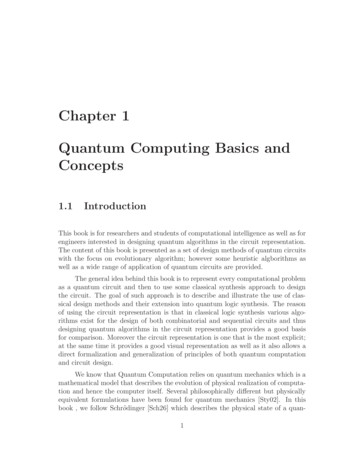
Figure 1: The explicit encoding vs. implicit encoding. An encoding isometryV is often embedded in a unitary U .1.2BasicsLet’s first explain what an encoding is. For quantum codes, weoften use linear encoding defined by an isometry V : Hl C H which satisfiesV † V 1, V V † P,(1)for P as the projector on the code space C H. Also we requiredim(H) dim(Hl ) so that there are redundancy to encode states.Which one is more fundamental, V or P for a code? It turnsout both are okay. A code definedPby V is explicit since it showsthe map ii 7 ψi i with V i ψi ihi for an orthonormalbasis { ii} of Hl , and a code defined by P is implicit since themap ii 7 ψi i is only described classically, and it still needsto construct V separately. For instance, the code 0i 7 000i, 1i 7 111i which encodes a qubit into three qubits is explicitlydefined by its encoding circuit. The code 0i 7 n 0i, 1i 7 n 1i which encodes a qubit into number states of an oscillatoris implicit since the encoding circuit is often not specified. Seefigure 1 for their differences. In general, for explicit encodingsthe physical space H contains the original logical space Hl , andfor implicit ones it is not the case.3
Now we shall discuss noise operators, or called error operators, which can disturb information in C by causing leakage toC H C or making changes in C itself. Do we have to correctthe noises? We don’t have to if we do not need the informationto be fully protected, depending on the tasks. For instance,the noises may be weak for some communication channels, socodes can be designed just to protect against particular typesof noises so that the fidelity of output can be high enough. Inother words, we do nothing for recovery. However, for error correction we need to apply a recovery channel, R, and also forerror detection we need to apply the projector P onto the codespace.For an error operator A, the simple correction scheme (i.e.recovery) is to apply its inverse A 1 . In quantum theory, weoften consider unitary operators or quantum channels definedby a set of Kraus operators. One central result of QEC is thatgiven a code C and a set of error Poperators {Ei }, which shallform a channel N with condition i Ei† Ei 1, the errors canbe corrected iffP Ei† Ej P cij P(2)for [cij ] as a non-negative matrix, known as coding state ρC . Therecovery is not by Ei but linear combination of them. Namely,the coding state ρC can be diagonalized with eigenvalues da , andthe condition will becomeP Fa† Fb P da δab P.(3)The recovery channel is defined by a set of operators Ra 1 F † . It can be easily checked thatadaRN (ρ) ρ, ρ C.4(4)
The condition above means that different Fa acting on P leadsto orthogonal spaces so they can be distinguished.Quantum error detection (QED) can be viewed as a simpleversion of QEC. The condition for QED of a channel isP Ei P ei P,(5)which is a weaker condition than QEC. This means that a codecan detect more errors than correct them.A crucial property of QEC is that if a code corrects a set {Ei },then it also corrects any operators in the linear span of {Ei } bythe same recovery R. So, strictly speaking, the correction is notabout a single channel; instead, it is about an operator space,which covers many more channels. This “linear-span” propertyhas profound consequences. For instance, usually we considercodes using many qubits, and we only need to consider errorson each qubit, and the spanning qubit errors are just the Paulioperators: X, Y, Z. Correcting Pauli errors will guarantee thecorrection of other error operators. As such, we often speak of“number of errors”, which refer to the weight of arbitrary errorsof the form n An for n as labels of qubits.The opposite of noise operators are logical operators, alsoknown as gates. Here we only consider unitary ones. A unitaryU acting on H is logical iff[U, P ] 0.(6)That is, it preserves the code space. The set of logical operators forms a group, usually SU (d), with the code space C as arepresentation of it. There are also hybrid operators which areboth logical and noisy: they lead to logical operations yet withleakages. Hybrid operators are dangerous for a code since they5
are not correctable, and they can determine the actual distanceof a code.The distance of a code dc is defined as the minimal “size”of operators that can lead to a logical operator. The notion ofdistance refers to distances among codewords ψi C. Higherdistance means the code is more robust against noises. Here“size” can be measured by various quantities depending on thecontexts. There are two basic settings: when H is of the form n Hn or the form n Hn . We often consider weight of operators with tensor-product forms, and power of operators for theother case. For instance, the weight of a tensor-product of Paulioperators n σn is the number of non-identity σs in it. Nowgiven a distance dc , it is clear to see (from the QEC condition)it means (dc 1) errors can be detected, while (dc2 1) errors canbe corrected.Let’s focus on codes with multiple qubits which are the common setting. A code of n qubits encoding k logical qubits withdistance d is denoted as [[n, k, d]], the double-bracket meaning“quantum” but here we use the simple notation [n, k, d]. A natural question is: are their any relations among n, k, d? It turnsout there are some tradeoffs from coding bounds, and the wellknown ones are Hamming bound, Singleton bound, and GilbertVarshamov (GV) bound. The Singleton bound says thatn k 2(d 1),(7)while the classical version of it is n k (d 1). The differencecomes from the fact: for qubits we need to correct both X andZ, but for classical bits we only need to correct Z. To be precise,let’s see how to prove it. Consider an orthonormalbasis { ii}P1for k qubits and the Bell state Φi 2k i iii of 2k qubits,6
and then apply the encodingisometry V to half of them. WeP10now have Φ i 2k i i, φi i for k n qubits. Divide the nqubits to groups of d 1, d 1, and n 2(d 1) qubits, withlabel A, B, and C. Label the other k qubits as R. Now thecode distance d means ρRA ρR ρA , ρRB ρR ρB . Usingentropy relations SAC SA SC , SBC SB SC , we will getk SR SC n 2(d 1). In other form, it isk(d 1) 1 2.nn(8)The Hamming bound and GV bound arise from a counting ofdistinct errors, which is, in order, an upper boundkdd 1 ( ) log 3 h( ),n2n2n(9)and a lower boundkdd 1 ( ) log 3 h( ),nnn(10)with h(x) the binary entropy of x. The Hamming upper boundis more tight than the Singleton upper bound, but the lateralso applies to degenerate code, which means some errors areequivalent and can be corrected by the same recovery scheme.We will show below that topological codes are highly degenerate,and this greatly benefits the design of good codes.1.3More: stabilizer codesFor multi-qubit codes, a large class of codes is the stabilizercodes, for which a code projector P is defined from a set of socalled stabilizers {Si }, which are low-weight product of Pauli7
operators and commuting. There is a nice group-theoretic description: the stabilizers form an Abelian group, the stabilizergroup, and for a code [n, k, d], there are (n k) stabilizer generators. The errors to consider are also low-weight product ofPauli operators, and correctable errors anti-commute with somestabilizers. The anti-commutation pattern forms the syndrome,and for non-degenerate stabilizer codes each error has distinctsyndrome. A signature of non-degenerate stabilizer codes is thatthe weight of stabilizers have to be larger than d since otherwisethe product of two errors Ea Eb can be a stabilizer, then Ea andEb cannot be distinguished (see the QEC condition). In this section, we will use examples to reveal features of stabilizer codes.From Singleton bound, the minimal n to encode a qubit withdistance 3 is 5. This is the so-called five-qubit code, or XZZXcode since the stabilizers are XZZX1, 1XZZX, X1XZZ,ZX1XZ, ZZX1X. It is non-degenerate. Each stabilizer can besplit as a product, e.g., XZZX1 (XY X11)(1XY X1), withXY X11 as a logical operator. By passing, this is actually fromthe cluster state. The code is implicit since we do not know theencoding circuit. To prepare the code, we can prepare a fivequbit cluster state by expressing it as a matrix-product statewith periodic boundary condition. We can also use XXXXXas a logical operator which anti-commutes with XY X11.More interesting codes will involve more qubits. We do notintend to review all known stabilizer codes since there are toomany. Below we survey some types of them, and these typesmay overlap. CSS codes: all stabilizers are product of X or product of Z.A CSS code can be constructed from two classical codes.An example is Shor’s 9-qubit code, with stabilizers of the8
form ZZ and n Xn , similar with the Hamiltonian of Isingmodel. topological (or local) codes: the physical support of H ison a regular manifold and the support of each stabilizeris geometrically local and a constant. Logical gates aretopological. Examples are toric code and color code, whichphysically are spin liquids. subsystem codes: the code space C is defined by a set ofnon-commuting local gauge operators, while a set of semilocal stabilizers also exist. The space has two parts C T G, with T as the true code space and G as a gauge spacethat does not encode information but participate the errorcorrection. An example is Bacon-Shor code, also physicallyknown as the quantum compass model. finite-rate LDPC codes: the encoding rate r nk staysfinite as n , and LDPC means low-density paritycheck, namely, each qubit is involved in a constant number of stabilizers, and each stabilizer involves a constantnumber of qubits (but may not be local). An example isthe hypergraph-product codes.The topological codes are famous since they are robust againstmany kinds of local noises. However, the redundancy is huge andthis is revealed from the boundkd2 O(n),(11)on 2D codes. It means the encoding rate r goes to zero if thedistance d increases with n. It’s beneficial to see how this isproved. First, it divides the system into three parts: correctable9
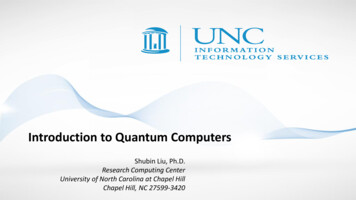
parts A and B, with the same size, and their boundary C thatis not correctable. This is similar with the proof of Singletonbound, and it shows k Rn2 for R as the linear size of A andB. Next it shows that R d which is not hard to see. Theproof is consistent with area law of entanglement which says thatthe entropy of a region scales with its boundary size, namely,information of a bulk is encoded in its boundary.Logical gates on topological stabilizer codes are also constrained. First recall that Pauli operators X, Y, Z with i1 forma group, called Pauli group, P, which is a projective representation of the Klein-four group Z2 Z2 . This extends to n-qubitcase as Pn . Now the so-called Clifford hierarchy is defined as aset of sets, and each set with integer label k 1, the ‘level’, isdefined asCk {U U P U † Ck 1 , P Pn C1 }.(12)The C2 is known as Clifford group, which contains Hadamardgate H, phase gate S, CNOT, and their products. Considerlogical gates from finite-depth local unitary (FDLU) operators,which do not change the topology of the code. It is shown thatD spatial topological stabilizer codes can support FDLU logicalgates from Clifford hierarchy for levels at most D. The proof isvery interesting and it uses a partition of the system into D 1correctable regions, Λj , different from the partition for the proofof encoding rate bound above. See figure 2 for a comparison.Consider a collection of D different Pauli logical operators Pj ,and require the support of Pj does not overlap with Λj . This isalways possible. The idea is to consider the commutator†Kj Pj† Kj 1 Pj Kj 1(13)for K1 U P1 U † with any FDLU U . Different Kj has different10
Figure 2: The partition for a topological stabilizer code for the proof ofencoding rate (left) and logical gates (right).supports, and it shows the support of KD is the last one: ΛD 1 .So logically KD 1 and it is easy to show U CD .Physically, it is not easy to understand the meaning of Kj .But we can treat gates in CD and lower as a set of order parameters that define the topological order of the code since FDLUoperations shall not change the topological order. For instance,for the toric code the FDLU logical gates include: Pauli gateswhich are loops, H gate and CNOT which are depth-one globaloperations, S gate which is slightly more complicated. The Pauliloops define the topological order of toric code, which has groundstate degeneracy as four robust against local perturbations. TheH gate, which maps between X and Z, is a duality of the codethat preserves the topological order. The same holds for S gatewhich maps between X and Y . The CNOT gate couples twotoric codes together while still preserves the topological order foreach of them. The above result shows that higher-dimensionaltopological order needs more order parameters to characterizeit, not just the Pauli operators.11
2Advanced topics: fault-tolerant quantumcomputingNow let’s move on to discuss how to use quantum codes for quantum computing. This is the framework of fault-tolerant quantum computing (FTQC), believed to be the inevitable model ofreliable quantum computing. We will analyze the notion of universality, what codes to use, the QEC algorithm, how to performgates, and how to carry out computing tasks.A computing process of FTQC looks like thisG1 · QEC · G2 · QEC · · ·(14)for G as various gates. We omit the initial state and final readout. The first issue is about universality, namely, what shall weachieve in FTQC. Universality means that any gate U SU (2n )for any n can be realized efficiently to arbitrary accuracy . Theefficiency means the cost of quantum computing, mainly thenumber of primary gates, scales as a polynomial of log 1 and n.The accuracy can be quantified by operator norm kU U 0 kor its equivalence which does not depend on initial states. Thekey point to note is that the accuracy can be arbitrarily small,otherwise it is not universal.To approximate U , which contains continuous rotation angles, we shall not use continuous-variable gates; instead, we use afew gates with fixed form, and these gates are “digital”. Namely,there exists universal gate set so that any U can be approximatedwell by a sequence of gates from a universal set. To prove theuniversality of a gate set is nontrivial, but here we only list a fewexamples: the set {H, T, CZ}, {H, CCZ}, {H, CS}, for CZ ascontrolled-Z, CCZ as controlled-CZ, CS as controlled-S, withS as phase gate. Given U SU (2n ), finding a sequence form12
of U 0 is a classical optimization problem that has been widelystudied. At the end, all gates in FTQC shall be these primarygates from universal gate sets.Note the gates above are logical and we still need to figure outhow to realize them physically. Recall that the logical part of Uis P U P . The simplest form of gate is the so-called transversalgatesU U1 U2 U3 · · ·(15)with each Un sandwiched by QECs on the site n. However, thereis a no-go theorem says transversal gates cannot be universal;probably because it is too good. An extension of it is the FDLUwhich was mentioned above. These gates do not spread outerrors too far due to the finite depth so do not jeopardize QEC.However, finding FDLU logical gates is difficult given a certaincode.At this point we shall mention the anyonic quantum computing, which realizes logical gates by braidings of non-Abeliananyons. Braidings are linear-depth local unitary circuits, so theycan spread out local errors to be nonlocal ones. QEC needs tobe done after each braiding to ensure fault tolerance, and this isnot an easy task in practice. We will review anyonic quantumcomputing separately.Now for codes and QEC, which codes to choose for FTQC?There shouldn’t be a unique answer since different codes havedifferent merits. We can just use a single code if it is powerfulenough, but so far no such code is known. So we have to usecombinations of codes. Some primary ways are as follows: Concatenation: use encodings in sequence. e.g., Shor’scode.13
Switching: use encodings alternatively. For stabilizer codes,this means to use stabilizer measurements to convert between codes. Augmentation such as state injection: use additional resources beyond the codes. e.g., magic-state injection forthe T gate which can be used for toric code FTQC.The errors encountered in different schemes are different, so theQEC are also different. However, a common thing is the physicalerror rate rp has to be below a threshold, rp , so that the logicalerror rate rl can be made arbitrarily small by increasing thedistance of the code. This is the content of the threshold theorem.Just like the classical repetition code, the noise on each bit shallnot be too strong in order for the code to be reliable.The QEC procedure becomes tedious for large codes suchas topological codes. A decoder is a classical algorithm whichis necessary to decide the recovery scheme from the syndrome.For degenerate codes, there could be various distinct decodersand finding optimal decoders is nontrivial. Decoders are oftenused in numerical studies.A well-studied setup for FTQC is based on (gauge) colorcode. We will not discuss the details here but the scheme isquite simple. Color codes are a family of 3D CSS codes andthere is a color code with transversal CZ and T gates, but notH gate. The idea is to use code switching to a gauge color codewhich has transversal H gate. However, the codes are 3D andthe weights of stabilizers are not so small. Compared with toriccode, no magic state is needed which is a great advantage ofcolor codes.Finally, we have to know how to perform a computing task.For short, quantum computing is just a sequence of gates, namely,14
a quantum circuit. However, we need to know how a circuit isdesigned and how it performs. This often requires some classical algorithms and this leads to the classical-quantum hybridparadigm. There are two types: a) loop-free: there is a classicalalgorithm A that design a quantum circuit Q. b) feed forward:there is a classical algorithm A that can change a quantumcircuit Q depending on the measurement output M from Q.Quantum machine learning is such an example. In addition, wecan also envision a fully quantum paradigm, but this is not wellunderstood yet.3Relevant theory: dynamical decoupling, error mitigation, randomized benchmarkingA universal FUQC is very powerful, and there is no hope to buildone within decades. Just like the classical case, there could bevarious types of non-universal computing devices that are alsouseful, such as simulators, detectors, sensors, calibrators, etc.These devices do not require powerful QEC but still can havesome ability to fight against decoherence or noises. Here wesketch some approaches.We can try to suppress errors instead of correcting them. Atechnique is known as dynamical decoupling (DD), which usesrapid time-dependent controls and relies on Magnus expansionof time-dependent evolution. The external noises is expected toaverage out when the control rate is faster than the time scaleof noisy processes. The noisy process L together with the DDscheme D shall be close with a unitary process U . For quantumcomputing, DD is used to extend the lifetime of qubits whilecompatible with execution of gates.15
Instead of dealing with evolution, the error mitigation (EM)technique focuses on observable. Expressing the ideal state asa linear combination of noisy ones, the ideal observable can beapproached by taking linear combination of noisy ones. Thisrequires to run the noisy circuit many times, each with differentnoise configurations. The number of samples is argued to beefficient with the desired accuracy of observable.Errors do not only arise from external noises. Imperfect physical operations to realize gates also introduce in errors. In QECwe often assume this kind of control errors can be treated asexternal errors, but this is not the case for other settings. Atechnique to calibrate and improve gates is known as randomized benchmarking (RB). The basic idea is to use random circuits composed with random gates that would do nothing if thegates were perfect, and then measure observable. From thesesamples it can extract the average gate infidelity. Furthermore,the gate operations may depend on a few parameters, and anoptimization is possible based on RB to increase the gate fidelityby tuning the parameters.4FrontiersThere are lots of frontiers, although the first-generation quantum computers (or simulators) are already in use, e.g., moderatescale optical lattices, superconducting qubit networks, linear optics networks, etc. These simulators are not fault tolerant.A frontier is to find better LDPC codes, as hinted by thecoding bounds. As we know, CSS codes are combinations ofclassical codes. So it is natural to consider combinations ofquantum codes. Some recent examples are homological prod16
uct codes, hypergraph product codes, fiber bundle codes, etc.The goal is to have both the encoding rate nk and distance dincreasing with the system size n. These codes are mainly constructed mathematically, and it is not clear yet what physicalphases of matter they correspond to (probably gapless phaseswith long-range interactions). Also FTQC with them just beginto develop.A subject we did not discuss is approximate codes which donot fully recovery logical states. This paradigm lies in betweenthe FTQC and noisy computing. There are some approximatecodes such as GKP code, VBS codes, holographic codes, etc, buta full theory of quantum computing with approximate codes isnot developed yet. These codes do not obey the standard codingbounds, but on the other hand, the accuracy of such computingis limited.Anyonic quantum computing is a setup people are trying torealize in labs, and there is a hope to achieve this via Majoranasystems in a decade. Although some non-braiding operationsare needed to achieve universality, this system could be betterthan others such as superconducting computers.A theoretical subject is about self-correcting codes. This ismotivated by the classical example: 2D Ising model. We can encode a classical bit in the magnetization, which is robust againstthermal noises below the critical temperature Tc . The encodingis a subsystem code, since we only need the sign of magnetization instead of its values. The 4D toric code is a self-correctingquantum code, which is physically a spin liquid, but clearly wecannot realize it easily in 3D. There is a hope to find new onesin fracton orders or finite-rate LDPC codes, which physicallyrely on non-thermal, glassy, or other mechanism instead of gas17
or liquid mechanism.5History, people, and storyAs we mentioned, the subject of QEC starts just a bit late thanquantum computing itself. The stabilizer framework was established in 1997 and becomes the main stream of quantum codes.Probably lots of computer or information scientists think theyare the only kind of quantum codes. Stabilizer states are very‘classical’, in the sense that they can be efficiently representedclassically, and operations that only change stabilizers to stabilizers can also be efficiently simulated on classical computers.The errors to deal with are Pauli X and Z, which is just two‘copies’ of errors instead of one for classical codes. But superposition of stabilizer states are not stabilizer states anymore, andthis is the origin of being quantum. Physicists are also developing non-stabilizer codes which are not so intuitive for computerscientists. Most likely, they will deviate from each other furtheraway in the near future, dividing the world of quantum codesinto stabilizer and non-stabilizer parts.The features of topological stabilizer codes were mainly studied by S. Bravyi, a leading theorist at IBM, around 2010. Theresults are, however, mostly negative regarding encoding rate,logical gates, self correction, etc. However, this motivates peopleto look for better codes with topological codes as an ingredientor mirror. He also works on many other subjects such as quantum algorithms, computational complexity, anyonic quantumcomputing, etc all with high-impact results. It is fair to say heis the kind of genius who is required to be there to clean up theway in the field of quantum computing, as commonly to be the18
case for any field.Another phenomena to notice is there are not many Chinesein the subject of QEC, given the large amount of researchers onquantum computing. This situation will change gradually sincequantum simulators will prove to be highly limited, and FTQCseems to be the right choice in the long run.References Daniel Gottesman, An Introduction to Quantum Error Correction and FaultTolerant Quantum Computation, arXiv:0904.2557. Barbara Terhal, Quantum Error Correction for Quantum Memories, Rev.Mod. Phys. 87, 307 (2015).Concept map19
veloped for two decades, just a little bit shorter than quantum computing itself. QEC is the most crucial part for quantum computing since it ensures the computation to be reliable, oth-erwise the output of a computing device is just crap. So every quantum computer scientist has to understand QEC and the framework of fault-tolerant quantum .