WIXLIB

6CHAPTER 1. QUANTUM COMPUTING BASICS AND CONCEPTSthe system in the state represented by Av. The overall process of the input statebeing evolved and measured can be seen as a vector-matrix multiplication. Theinterested reader can find more information about the Hilbert space and quantumprobabilistic systems in [WG98, HSY 04, YHSP05].In the above introduced dirac notation eq. 1.4 is rewriten to:(1.5) wi A viObserve the introduction of the bra-ket notation considerably simplified eq. 1.4.1.3.4Kronecker ProductThe combination of qubits into a multi-qubit system is mathematically given by theKronecker multiplications; for a two-qubit system we obtain (using the Kroneckerproduct [Gru99, Gra81, NC00]) the states represented in eq. 1.6: 01 0100 11 10i 00i 10100000 00 0001 01 11i 01i 01101010 (1.6) Similarly for Operators, the Kronecker product exponentially increases thedimension of the space: 1 1 0 0 1 1 1 0 0 11 11 0 (1.7) W H 0 12 1 12 0 0 1 1 0 0 1 1This operation is shown in Figure 1.1.Assume that qubit a (with possible states 0i and 1i) is represented by Ψa i αa 0i βa 1i and qubit b is represented by Ψb i αb 0i βb 1i . Each of them isrepresented by the superposition of their basis states, but put together the characteristic wave function of their combined states will be:

1.3. MATHEMATICAL PRELIMINARIES TO QUANTUM COMPUTING7HFigure 1.1: Circuit representing the W H operation Ψa Ψb i αa αb 00i αa βb 01i βa αb 10i βa βb 11i(1.8)with αa and βb being the complex amplitudes of states of each EP respectively. Asshown before, the calculations of the composed state are achieved via the Kroneckermultiplication operator. Hence come the quantum memories with extremely largecapacities mentioned earlier and the requirement for efficient methods to calculatesuch large matrices.1.3.5Matrix TracePA trace of a matrix is defined as tra(U) i Dii and as it will be seen the conceptof trace is used in the measurement operation in quantum computing. In particularit is required when dealing with ensemble systems [CFH97, NC00] and estimatingtheir state. Such systems are represented by density matrices of the form:nn(1.9)ρ 2XiwithP2niαi ψi ihψi αi 2Xipi ψi ihψi pi 1, α being the complex coefficient such that αi 2 pi .The trace operator represents the possible observable states of a quantum system.Any quantum state φi when observed collapses according to the applied measurement resulting in α φi p φihφ , with p being the probability of observing the state φi from the set of all possible output states. Thus representingthe overall state ofP2na quantum system can be represented as the trace i 0 pi iihi with pi being theprobability of observing the state ii.

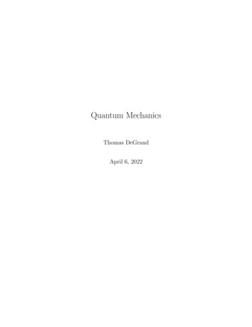
81.41.4.1CHAPTER 1. QUANTUM COMPUTING BASICS AND CONCEPTSQuantum MechanicsBohr Particle ModelThe term ”quantum” describes the fact that the EP’s can be observed (measured)only in distinct energetic states and while moving from one state to another a quantified amount of energy is either emitted or absorbed. A closer look at the Bohrmodel of the atom will explain these notions even more. The example we are usinghere is based on the simplest of all atoms, the Hydrogen (H) atom. As all atoms, theHydrogen atom (H) is composed of a nucleus and electrons orbiting around it, butH has only one electron (e). The electron can be only on orbits of certain allowedradii. When e is on the orbit that is closest to the nucleus then the atom is in the”ground state”.The electron can change orbits; going from a lower orbit to a higher one requiresabsorption of some energy and leaving an orbit for a lower one is characterized byemitting a quantum of energy from the electron. The energy levels that the electroncan visit are characterized by the following equation:(1.10)En (Rh ) 1n2 where Rh is the so-called Rydberg constant (2.18 10 18 J) and n is the principlequantum number corresponding to different allowed orbits of the electron. Thedifference of energy E associated with ”orbits-jumping” can be expressed as thedifference between the energy of the electron on the initial Ei and the final Ef orbit:(1.11) E Ef EiMax Planck has deduced that the energy of electrons comprising the electro-magneticradiation is a function of frequency, from where his famous formula comes:(1.12) E hν Rh11 22nfni!where h is the Planck constant (6.63 x 10-34 Js) and v is the frequency of the emittedlight (Figure 1.2).

91.4. QUANTUM MECHANICSFigure 1.2: Bohr model of the atom (nucleus, orbiting electrons). Shown are lightcolors respective to the electron orbit transitions.1.4.2Quantum Model of Elementary ParticleThis brief look into the physical background should be completed by the fact thatBohr’s model of atom assumed that the electron is orbiting the nucleus similarlythe Earth is orbiting around the Sun, which violates the Heisenberg uncertaintyprinciple of Quantum Mechanics [Cas]. This principle states that the position andthe momentum of an EP cannot be simultaneously determined with certainty. Inparticular in quantum mechanics, any elementary particle has the propertyp that theroot-mean-square deviation of the position x from the mean x hx2 i hxi2(where h·i representsx x ) and root-mean-square of the momentum p from thepmean p hp2 i hpi2 multiplied together is never smaller than 2 . This is alsoexpressed by the commutator:(1.13)[x, p] iℏThe introduction of these unusual properties was required to correctly describe theQM system (sometimes also referenced as a ”failure” of the classical Bayesian statistics [You95]) and to allow predicting states of Physical Quantum Systems.Example 1.4.2.1 Two-Slit experimentIn the two-slit experiment, the dual nature of EP was shown. The experimentconsists of the emitter (device firing EP on a screen), of the screen with two holesand of the detector. Figure 1.5 illustrates the experimental setting. The system

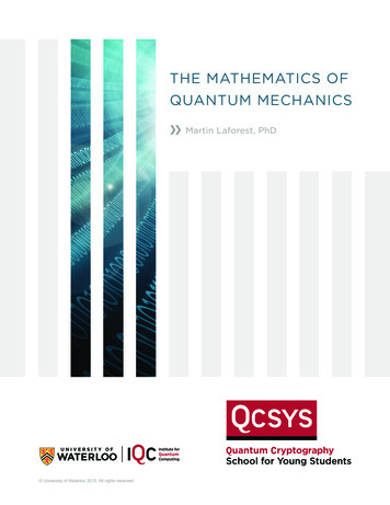
10CHAPTER 1. QUANTUM COMPUTING BASICS AND CONCEPTSFigure 1.3: The measured number of electrons on the detector screen with top slitor the bottom slit open (thin lines). The expected probability when both slits areopen (thick line).is setup so that the electrons detected by the detector have to travel through theopen holes (the screen is thick enough to stop the electrons completely). Whenonly one of the two slits is open and the observer looks at (measures) the projectionof fired particles on the detector, the distribution of their locations is proportionalto a linear trajectory through the opened slit (photons behave like particle). Theparadox shows up when both the slits are opened.Figure 1.3 shows the detection screen and the number of electrons measured wheneither the top or the bottom slit is open. Two curves show the distribution ofparticles on the detector screen either with top or with the bottom slit open. Thethick curve is an expectation of what should be the particle distribution with bothslits opened based on the classical probability theory. What appears to be a classicalprobabilistic distribution of particles with only one of both slits open, is transformedto an interference pattern with both slits open (Figure 1.4), not obtainable usingclassical statistics.When this measurement was made the problem was to interpret it and to decidewhereas EP’s travel in space on a straight line (as particles) or if they have waveproperties. The problem was to determine how an EP (electron or photon) hasthe particle characteristics (mass and speed) when measured and could behave as awave at the same time? The dual nature problem is solved by the supposition thatthe EP is a particle while the measurement is performed, and the EP behaves likea wave while not.According to Figure 1.5 it is not possible to decide whereas a particle traveledthrough one, two or both slits simultaneously because the measurement does notallow determining it. If a measurement of particles is done on the screen, the result

1.4. QUANTUM MECHANICS11Figure 1.4: Results of measurement of particles position when both slits of the screenare open.Figure 1.5: Schematic representation of the two-slit experiment. Left is the emitterand on the right is the detector (film). In the middle is the barrier with two holes.

12CHAPTER 1. QUANTUM COMPUTING BASICS AND CONCEPTSwill yield 50% of particles through left slit and 50% through the right slit. Theconsequence of these observations is the fact that while recording probabilities ofdetecting an electron in the interference pattern, the probabilities of observation ofa given state can be smaller than in the standard Bayesian probabilistic model! Thisimplies the following contradictory equation 1.14 [You95].(1.14)P (x) P (x slit1 ) P (x slit2 ) P (x slit1 )where P(x) is the probability of measuring a particle on position x. The solutionto this problem was the introduction of the concept of the complex probabilityamplitudes because such amplitudes can cancel each other. The system describe byeq. 1.14 is then mathematically a set of functions mapping real physical states fromHilbert space H into a complex space C:(1.15)Ψ:S Cwhere S is the physical space of states and C is complex vector space, respectively.As will be seen later, the functions from the set described by eq. 1.15 are the wavefunctions that represent non-trivial states of the quantum system. This state ofa particle traveling through both slits is defined as the ”superposed” state of thesystem. For one-particle system this superposition is a result of all its possiblestates that it is measured for. Its complex probability amplitude α is related to theclassical probability p of measuring this system in a particular state by α 2 p. Ina system of n particles (called also the quantum register), the system constitutes asuperposition of m n states where m is the number of states of each elementaryunit of this system.1.4.3Schrödinger equationThe general solution for quantum mechanical events is given by the Schrödingerequation:(1.16)iℏd ψi H ψidtwith ℏ being the Planck constant [Pla] and H being the Hamiltonian of the system.A Hamiltonian represents the observable corresponding to the total energy of the

131.4. QUANTUM MECHANICSsystem. In particular, the possible observable states are represented by the spectrumof the Hamiltonian [Dir84]. This general equation describes the natural evolutionof a quantum system. The ℏ constant can be absorbed into the Hamiltonian H.The Hamiltonian H can for example represent a particle that exists in the infiniteone-dimensional potential such as the Simple Harmonic Oscillator (SHO) [MV76]p2 12 mω 2 x2 where p is the momentum, m is themodel with Hamiltonian H 2mmass, x is the position and ω is the angular velocity. The Schrödinger equation forSHO takes the form of: ℏ d2 ψn (x) 1 2 βx ψn (x) Eψn (x)2m dx22(1.17)qβwhere V (x) is the potential well with ω (and β being the springmconstant). In general the solution that one obtains when solving for physical systemsis a solution to eq. 1.16 which is of the form:1βx22 ψ(t)i e iHt/ℏ ψ(0)i(1.18)or more clearly as(1.19) ψ(t)i e inωt ψ(0)iwith ω being the angular frequency and n being the index of distinct non-degeneratequantum states. From the eq. 1.19 and with respect to previous stipulations (orpostulates of quantum mechanics) it can be observed that the resulting state is adistribution of corresponding probabilities pn over the set of eigenstates n [MV76].For more details, this particular problem has all solutions represented by Hermitepolynomials [MV76, Wey32], however it is not the focus of this book.1.4.4Superposition of quantum statesThe previous descriptions introduced a very unique phenomena: while a particlebehaves as a wave it can be simulateneously in various basis states but when it ismeasured (as in the two-slit experiment) the basis state reveals it self a physicallyobservable unique state. The state illustrated by eq. 1.19 is also called the quantumsupperposition of states because a single physical particle contains a multitude of

14CHAPTER 1. QUANTUM COMPUTING BASICS AND CONCEPTSobservable staes that have a finite probability to collapse onto the orthonormal basesstates. A more understandable explanation is to represent the quantum state as astate that is build of component observable states (with particular probabilities)and that when observed will be seen as one of the observables with the associatedprobability.Let’s illustrate the superposition phenomena by work done in [MMKW96]. Inthis experiment described is the creation of a ”Schrödinger cat” state of an atom.The ”Gedankenexperiment” of Schrödinger was to place a living cat into a superposition of being alive and dead. These superposed states in QM are described bya wave function. The cat state can be described in these terms as follows:(1.20) Ψi i i 2where i and i refer to the states of a living and dead cat, respectively. Once againthis situation is not ”realistic” in our macro-world, however appropriate for the QM.The interpretation of the general equation 1.20 is that for each measurement of thesystem described by it there is 50% chance to find the system in state i and a 50%chance to find the system in state i. This can be formalized in Dirac’s notationas:(1.21)(1.22)Ψ α i β i11 i i22with(1.23) α 2 β 2 1Where α and β are in general complex amplitudes associated with each measuredstate, and α 2 αα where α (a ib) (a ib) is a complex conjugate of α.Thus both states i and i will be observed when measured with probabilities α2 and β 2 respectively. This interpretation of the system defined by (1.22), shows thatany quantum system can be represented by a wave function describing all possiblestates of the system (here we assume two orthonormal states i and i) by usingcomplex probabilities (here α and β). The complex probabilities are restricted onlyby the second equation in (1.23), and the observables of this quantum system arevalued in the range of {0, 1}.

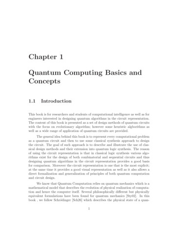
1.4. QUANTUM MECHANICS15Figure 1.6: The Bloch sphereThe above representation is another notation of a Euler parametrized 3D rotation. The general state of a qubit rotation is given in eq. 1.24. Observe howdemonstrated in this equation, a global phase eiρ is visible, but in general it isignored during the computation with qubits as it can be easily factored out andmoreover, upon measurement it is completely destroyed. θθcos 2θ e iφ sin θ2i(ρ φ)iρ(1.24) ψi e cos 0i esin 1i R(ρ, φ, θ) ecos θ2eiφ sin 2θ22iρThe equation 1.24 is more clearly visualized on a sphere, commonly known asthe Bloch sphere. This representation is usefull situated to show the state of a singlequbit but does not allow to represent multiple qubits due to entanglement and thesupperposition. The Bloch sphere is shown in Figure 1.6.Now, stepping back to [You95], if instead of a cat we consider some of alkali-like ionssuch as 40Ca , 24Mg or 198Hg which do not have a third electronic ground stateavailable for the auxiliary level (thus can be directly used for quantum permutativecomputing) [MMKW96], the equations (1.22) and (1.23) would represent the wavefunction of an ion where i and i are two distinct energetic states.As mentioned earlier in this section (and as will also be seen in Section 1.5), operations on single trapped ions have been already implemented [MMK 95, MMKW96,MML 98, WMI 05]. This technique consists in trapping in an Electro-Magneticfield one or more ions and using laser beams setting these ions into certain states.Applying a well-determined sequence of laser pulses on particular ions in the trap,one can achieve such gates as NOT (an inverter of classical logic design). Again thesetting of ions is represented by jumps of electron on their orbits and emitting or absorbing quanta of energy. It also allows realizing one-qubit, two-qubit or even three

16CHAPTER 1. QUANTUM COMPUTING BASICS AND CONCEPTSqubit gates. However, no large-scale quantum computer was yet experimentallycreated using ion-traps.1.5From Quantum Mechanics to Quantum LogicIn the Section 1.4, the example of implementation of a quantum computer wasmentioned: the trapped ions in the EM field interacting with laser beams. Thishas for consequence the changes of states of the ions such as moving from groundstate to an excited state by an electron jump from a lower orbit to a higher one.But electrons are more complicated than just quantum energy collectors and theirwave functions are more complex because they depend on three parameters besidethe principle quantum numbers; the orbital quantum number ”l”, the magneticquantum number ”m” and the spin ”S”. While parameters l and m determinethe angular dependence, the S determines the internal electron rotation. For ourexplanation it is only important to know that the S number is often used to representbasis states in a Quantum Computation because the hydrogen atom can have onlytwo values 12 of spin. Consequently, using spin rotations for the basis implies towork directly with the two-valued (binary)quantum logic. Now, considering the spinS value as the basis, a quantum operator on an atom will result in a rotation of theelectron spin. Consequently all single qubit operations can be expressed as rotationsby certain angles [NC00].Moreover to build a quantum computer a multi-qubit system (also called quantumregister) requires to be defined and analyzed. Beside the quantum register definitionaddtional operations such as measurement have to be explained.1.5.1Multi-Qubit SystemTo illustrate these important properties let’s have a look on a more complicatedsystem with two quantum particles a and b represented by ψa i α0 0i βa 1i and ψb i αb 0i βb 1i respectively. For such a system the problem space increasesexponentially and is represented using the Kronecker product [Gru99]. αα01 α0 β1 α1α0 (1.25) ψa i ψb i β0 α1 β1β0β0 β1Thus the resulting system is represented by ψa ψb i αa αb 00i αa βb 01i βa αb 10i βa βb 11i (1.8) where the double coefficients obey the unity(completeness) rule and

171.5. FROM QUANTUM MECHANICS TO QUANTUM LOGICeach of their square powers represents the probability to measure the correspondingstate

sition from quantum physics to quantum computing. We also introduce quantum computing models, necessary to understand our concepts of quantum logic, quan-tum computing and synthesis of quantum logic circuits. The Section 1.3 introduces some mathematical concepts and theories required for