WIXLIB

ADAPTIVELY SCALING THE METROPOLIS ALGORITHM5Throughout this paper we use the notation θt for the proposal generated by the4Metropolis chain under proposal kernel Jγ (·, θt ) and denote by t θt θt , theproposed jumping distance.2.2. Optimization of the proposal kernel after one set of simulationsFollowing Andrieu and Robert (2001), we define the objective function thatwe seek to maximize adaptively as[] 4h(γ) E H(γ, θt , θt ) H(γ, x, y)π(x)Jγ (x, y)dxdy. (2.2)Rd RdWe start our procedure by choosing an initial proposal kernel Jγ0 (·, ·) and runningthe Metropolis algorithm for T steps. We use the T simulation draws θt and theproposals θt to construct the importance sampling estimator of h(γ), TH(γ, θt , θt ) · wγ γ0 (θt , θt )4ĥT (γ γ0 ) t 1 T, γ Γ,(2.3) t 1 wγ γ0 (θt , θt )or the mean estimatorT4 1 ˆĥT (γ γ0 ) H(γ, θt , θt )wγ γ0 (θt , θt ), γ Γ,T(2.4)t 1where4wγ γ0 (θ, θ ) Jγ (θ, θ ),Jγ0 (θ, θ )(2.5)are the importance sampling weights. On the left side of (2.3) the subscript Temphasizes that the estimate comes from T simulation draws, and we explicitlycondition on γ0 because the importance sampling weights require Jγ0 .We typically choose as objective function the expected squared jumped distance H(γ, θ, θ ) kθ θ k2Σ 1 αγ (θ, θ ) (θ θ )t Σ 1 (θ θ )αγ (θ, θ ), whereΣ is the covariance matrix of the target distribution π, because maximizing thisdistance is equivalent to minimizing the first-order autocorrelation in covariancenorm. We return to this issue and discuss other choices of objective function inSection 2.4. We optimize the empirical estimator (2.3) using a numerical optimization algorithm such as Brent’s (see, e.g., Press, Teukolski, Vetterling andFlannery (2002)) as we further discuss in Section 2.6. In Section 4 we discussthe computation time needed for the optimization.2.3. Iterative optimization of the proposal kernelIf the starting point, γ0 , is not in the neighborhood of the optimum, thenan effective strategy is to iterate the optimization procedure, both to increase

6CRISTIAN PASARICA AND ANDREW GELMANthe amount of information used in the optimization and to use more effectiveimportance sampling distributions. The iteration allows us to get closer to theoptimum and not rely too strongly on our starting distribution. We explore theeffectiveness of the iterative optimization in several examples in Section 4. Inour algorithm, the “pilot data” used to estimate h will come from a series ofdifferent proposal kernels. The function h can be estimated using the methodof multiple importance sampling (see Hesterberg (1995)), yielding the followingalgorithm based on adaptively updating the jumping kernel after steps T1 , T1 T2 , T1 T2 T3 , . . . For k 1, 2, . . .1. Run the Metropolis algorithm for Tk steps according to proposal rule Jγk (·, ·). ), . . . , (θ Save the sample and proposals, (θk1 , θk1kTk , θkTk ).2. Find the maximum γk 1 of the empirical estimator h(γ γk 1 , . . . , γ0 ), definedas k Ti t 1 H(γ, θit , θit ) · wγ γk 1 ,.,γ0 (θit , θit )i 1, (2.6)ĥ(γ γk 1 , . . . , γ0 ) kTi t 1 wγ γk 1 ,.,γ0 (θit , θit )i 1where the multiple importance sampling weights are4wγ γj ,.,γ0 (θ, θ ) jJγ (θ, θ )i 1 Ti Jγi 1 (θ, θ ),j 1, . . . , k.(2.7)We are treating the samples as having come fromof j components j a mixture ) 1,iwγ γk 1 ,.,γ0 (θit , θit1, . . . , k. The weights satisfy the condition ki 1 Tt 1and are derived from the individual importance sampling weights by substitutingJγ ωγ γj Jγj in the numerator of (2.7). With independent multiple importancesampling, these weights are optimal in the sense that they minimize the varianceof the empirical estimator (see Veach and Guibas (1995, Theorem 2)), and ournumerical experiments indicate that this greatly improves the convergence of ourmethod. It is not always necessary to keep track of the whole chain and proposals, quantities that can become computationally expensive for high-dimensionaldistributions. For example, in the case of random walk Metropolis and ESJD objective function, it is enough to keep track of the jumped distance in covariancenorm and acceptance probability to construct the adaptive empirical estimator.We discuss these issues further in Section 3.2.4. Choices of the objective functionWe focus on optimizing the expected squared jumped distance (ESJD), whichin one dimension is defined as[ [][]]22 ESJD(γ) EJγ θt 1 θt EJγ EJγ θt 1 θt (θt , θt )[] EJγ 2t · αγ (θt , θt ) 2(1 ρ1 ) · Var π (θt )

ADAPTIVELY SCALING THE METROPOLIS ALGORITHM7and corresponds to the objective function H(γ, θt , θt ) 2t · αγ (θt , θt ). Maximizing the ESJD is equivalent to minimizing first-order autocorrelation, whichis a convenient approximation to maximizing efficiency as we have discussed inSection 1.2.For d-dimensional targets, we scale the expected squared jumped distanceby the covariance norm and define the ESJD as[][]4ESJD(γ) EJγ kθt 1 θt k2Σ 1 E k t k2Σ 1 αγ (θt , θt ) .This corresponds to the objective function, H(γ, θt , θt ) k t k2Σ 1 αγ (θ, θ ) ( t )t Σ 1 t αγ (θt , θt ), where Σ is the covariance matrix of the target distributionπ. The adaptive estimator (2.6) then becomes4ĥ(γ γk , γk 1 , . . . , γ1 ) k Tii 1 2t 1 k it kΣ 1 αγi (θit , θit ) · wγ γk ,.,γ1 (θit , θit ). k Ti t 1 wγ γk ,.,γ1 (θit , θit )i 1(2.8)Maximizing the ESJD in covariance norm is equivalent to minimizing the lag-1correlation of the d-dimensional process in covariance norm,[](2.9)ESJD(γ) EJγ kθt k2Σ 1 .When Σ is unknown, we can use a current estimate in defining the objectivefunction at each step. We illustrate this in Sections 4.2 and 4.4.For other choices of the objective function already studied in the MCMCliterature, see Andrieu and Robert (2001). In this paper we consider two optimization rules: (1) maximizing the ESJD (because of its property of minimizingthe first-order autocorrelation) and (2) coercing the acceptance probability (because of its simplicity).2.5. Convergence propertiesFor fixed proposal kernel, under conditions on π and Jγ such that the Markovchain (θt , θt ) is φ irreducible and aperiodic (see Meyn and Tweedie (1993)), theratio estimator ĥT converges to h with probability 1. For example, if Jγ (·; ·) ispositive and continuous on Rd Rd , and π is finite everywhere, then the algorithmis π-irreducible. No additional assumptions are necessary to ensure aperiodicity.In order to prove convergence of the maximizer of ĥT to the maximizer of h, somestronger properties are required.Proposition 1. Let {(θt , θt )}t 1:T be the Markov chain and set of proposals generated by the Metropolis algorithm under transition kernel Jγ0 (·, ·). If the chain{(θt , θt )} is φ-irreducible, and ĥT (· γ0 ) and h are concave and twice differentiable

8CRISTIAN PASARICA AND ANDREW GELMANeverywhere, then ĥT (· γ0 ) converges to h uniformly on compact sets with probability 1, and the maximizers of ĥT (· γ0 ) converge to the unique maximizer ofh.Proof. The proof is a consequence of well-known theorems of convex analysisstating that convergence on a dense set implies uniform convergence and consequently convergence of the maximizers; this can be found in Geyer and Thompson(1992).In general, it is difficult to check the concavity assumption for the empiricalratio estimator, but we can prove convergence for the mean estimator.Proposition 2. Let {(θt , θt )}t 1:T be the Markov chain and set of proposalsgenerated by the Metropolis algorithm under transition kernel Jγ0 (·, ·). If thechain {(θt , θt )} is irreducible, and the mapping γ H(γ, x, y)Jγ (x, y), γ Γis continuous, and for every γ Γ there is a neighborhood B of γ such that[ ] Jφ (θt , θt )EJγ0 sup H(φ, θt , θt ) ,(2.10)Jγ0 (θt , θt )φ Bthen hT (· γ0 ) converges to h uniformly on compact sets with probability 1.Proof. See the Appendix.The convergence of the maximizer of hT to the maximizer of h is attainedunder the additional conditions of Geyer (1994).Theorem. (Geyer (1994, Theorem 4)) Assume that (γT )T , γ are the uniquemaximizers of (hT )T and h, respectively, and they are contained in a compact set.If there exist a sequence ²T 0 such that hT (γT γ0 ) supT (hT (γT γ0 )) ²T ,then γT γ .Proposition 3. If the chain {(θt , θt )} is φ-irreducible and the objective functionis the expected squared jumped distance, H(γ, x, y) ky xk2Σ 1 αγ (x, y), thenthe mean empirical estimator hT (γ γ0 ) converges uniformly on compact sets forthe case of random walk Metropolis algorithm with proposal kernel Jγ,Σ (θ , θ) exp( kθ θ k2Σ 1 /(2γ 2 )).Proof. See the Appendix.Remark. We used both the mean and the ratio estimator for our numericalexperiments, but the convergence appeared to be faster than Andrieu and Robert,and the estimates more stable for the ratio estimator (see Remark 1 below formore details).The infinite adaptation version can be proved to converge under some additional restriction, Haario, Saksman and Tamminen (2001) and Roberts andRosenthal (2006).

ADAPTIVELY SCALING THE METROPOLIS ALGORITHM9Proposition 4. Let π be a distribution function with a compact support S Rd .Consider the infinite adaptation version of the algorithm with Gaussian proposalkernel (see Section 3) with Tn . Then the Markov chain is ergodic and theWeak Law of Large Numbers holds for any bounded measurable function.Proof. The proof is a consequence of Proposition 1 and Roberts and Rosenthal(2006) Corollary 11 and remarks. By definition π has a compact support andΓ is a compact set, and we can take λ as the finite Lebesgue measure restrictedto the the product space S Γ. The proposal kernels are multivariate normals,which ensures that for fixed γ Γ, Pγ is ergodic for π(·), and that the densityis continous and bounded. By Proposition 1 for large n, γn converges to γ a.s.,which ensures that the diminishing adaptation condition of Theorem 5 is satisfied.Since empirical estimates of the covariance matrix change at the nth iterationby only O(1/n), it follows that the diminishing adaptation condition is satisfiedfor the covariance matrix. Compact support and convergence of the parameteralso ensures that simultaneous uniform ergodicity condition from Theorem 5holds which, in conjunction with Theorem 23 (Weak Law of Large Numbers),concludes the proof. Clearly, the ESJD is uniformly bounded, thus the Law ofLarge Numbers applies and, for Tn sufficiently large, γn converges to γ .Remark. One can also choose the adaptation times Tn to be the regeneration times of the Markov chain (identified by enlarging the state space with anatom) as demonstrated in Brockwell and Kadane (2005). This guarantees the convergence of the estimators at the n rate.2.6. Practical optimization issuesRemark 1. The ratio estimator (2.3) preserves the range of the objective function H(·), and has a lower variance than the mean estimator if the correlationbetween the numerator and denominator is sufficiently high (see Cochran (1977)).Other choices for the empirical estimator include the mean estimator hT and estimators that use control variates that sum to 1 to correct for the bias (see, forexample, the regression and difference estimators of Hesterberg (1995)).Multiple importance sampling attempts to give high weights to individualproposal kernels that are close to the optimum. For more choices for the multipleimportance sampling weights, see Veach and Guibas (1995).Remark 2. For the usual symmetric kernels (e.g., normal, Student-t, Cauchy)and objective functions it is straightforward to derive analytical first and secondorder derivatives and run a few steps of a maximization algorithm that incorporates the knowledge of the first and second derivative (see, e.g., Press et al.(2002), for C code) or as already incorporated in the R function optim(). If

10CRISTIAN PASARICA AND ANDREW GELMANanalytic derivatives do not exist or they are expensive to compute, then a gridmaximization centered on the current optimal estimated is recommended.Remark 3. Guidelines that ensure fast convergence of the importance sampling estimator In (h) ni 1 h(Xi )[(gγ (Xi ))/(gγ0 (Xi ))] of I(h) Egγ [h(X)] based onthe proposal distribution gγ0 (·) are presented in Robert and Casella (1998): theimportance sampling distribution gγ0 should have heavier tails than the true distribution; minimizing the variance of importance weights minimizes the varianceof In (h).3. Implementation with Gaussian KernelFor the case of a random walk Metropolis with Gaussian proposal densityJγ,Σ (θ , θ) exp[ (kθ θ k2Σ 1 )/(2γ 2 )], the adaptive empirical estimator (2.8)of the ESJD is k Ti2 2t 1 k it kΣ 1 α(θit , θit ) · wγ γk ,.,γ1 (k it kΣi 1 )i 14iĥ(γ γk , γk 1 , . . . , γ1 ) k Ti2t 1 wγ γk ,.,γ1 (k it kΣ 1 )i 1iwhereexp( x/(2γ 2 ))/γ d.wγ γk ,.,γ1 (x) kd2i 1 Ti exp( x/2γi )/γi(3.1)For computational purposes, we program the Metropolis algorithm so that it givesas output the proposed jumping distance in covariance norm k it kΣ 1 and theiacceptance probability. This reduces the memory allocation for the optimizationproblem to one dimension, and the reduction is extremely important for highdimensions where the alternative is to store d T arrays. We give here a versionof our optimization algorithm that keeps track only of the jumped distance incovariance norm, the acceptance probability, and the sample covariance matrix.1. Choose a starting covariance matrix Σ0 for the Metropolis algorithm, for example a numerical estimation of the covariance matrix of the target distribution.2. Choose starting points for the simulationand some initial scaling for the pro posal kernel, for example cd 2.38/ d. Run the algorithm for T1 iterations,saving the simulation draws θ1t , the proposed jumping distances k 1t kΣ 10 ). Optionally,in covariance norm, and the acceptance probabilities α(θ1t , θ1tconstruct a vector consisting of the denominator of the multiple importancesampling weights and discard the sample θ1t .

ADAPTIVELY SCALING THE METROPOLIS ALGORITHM113. For k 1, run the Metropolis algorithm using proposal kernel Jγk Σk . Updatethe covariance matrix using the iterative procedure)(TkΣk (i, j)Σk 1 (i, j) 1 Ttotal)(Tk 1θkt θjt (Ttotal Tk )θ̄k 1,i θ̄k 1,j Ttotal θ̄ki θ̄kj Ttotalt 1where Ttotal T1 · · · Tk , and update the scaling using the adaptive algorithm. We must also keep track of the d-dimensional mean, but this is notdifficult since it satisfies a simple recursion equation. Optionally, iterativelyupdate the denominator of the multiple sampling weights.4. Discard the sample θkt and repeat the above step.In updating the covariance matrix we can also use the greedy-start procedure using only the accepted jumps (see Haario et al. (1999)). For random walkMetropolis, analytic first and second order derivatives are helpful in the implementation of the optimization step (2) (e.g., using a optimization method), andcan be derived analytically. In our examples, we have had success updating theproposal kernel every 50 iterations of the Metropolis algorithm, until approximateconvergence.4. ExamplesIn our first three examples we use targets and proposals for which optimalproposal kernels have been proposed in the MCMC literature to demonstratethat our optimization procedure is reliable. We then apply our method on twoapplications of Bayesian inference using Metropolis and Metropolis within Gibbsupdates.4.1. Independent normal target distribution, d 1, . . . , 100We begin with the multivariate normal target distribution in d dimensionswith identity covariance matrix, for which the results from Gelman, Roberts andGilks (1996) and Roberts, Gelman and Gilks (1997) regarding the choice of optimal scaling apply. This example provides some guidelines regarding the speed ofconvergence, the optimal sample size, and the effectiveness of our procedure fordifferent dimensions. In the experiments we have conducted, our approach outperforms the stochastic Robbins-Monro algorithm, as implemented by Atchadéand Rosenthal (2003). These are well-known recursive algorithms, used to solvean equation h(γ) 0 where h is unknown, but can be estimated with a noise.Figure 6.1 shows the convergence to the maximum of the objective functionof the adaptive optimization procedure for dimensions d 1, 10, 25, 50, and

12CRISTIAN PASARICA AND ANDREW GELMANFigure 6.1. Convergence to the optimal value (solid horizontal line) at eachstep k of the adaptive optimization procedure,given seven equally spaced starting points in the interval [0, 3 2.38/ d], T 50 iterations per step, forthe random walk Metropolis algorithm with multivariate standard normaltarget of dimensions d 1, 10, 25, 50, and 100. The second and thirdcolumn of figures show the multiple importance sampling estimator of ESJDand average acceptance probability, respectively.100, as well as the corresponding values of the multiple importance samplingestimator of ESJD and average acceptance probability.When starting from very small values, the estimated optimal scale showssome initial high upward jumps. In order to eliminate high amplitude jumpsand slow convergence, the optimization could be restricted to the set where thevariance of the importance sampling weights is finite:}{(4.1)γ 0 γ 2 2 max γi2 .i 1:k

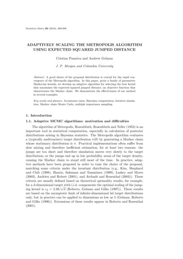
ADAPTIVELY SCALING THE METROPOLIS ALGORITHM13Figure 6.2. Convergence of the adaptive optimization procedure using asobjective the coerced average acceptance probability (to the optimal acceptance value from Figure 6.1). The second and third column show the multiple importance sampling estimator of the ESJD and average acceptanceprobability, respectively. Convergence of the optimal scale is faster than optimizing ESJD, although not necessarily to the most efficient jumping kernel(see Figure 6.3).In order to compare our algorithm with the stochastic Robbins-Monro algorithm, we have also coerced the acceptance probability by estimating the averageacceptance probability using the objective function H(x, y) αγ (x, y) and thenminimizing a quadratic loss function h(γ) (αγ (x, y)Jγ (x, y)dydx α )2 ,where α is defined as the acceptance rate corresponding to the Gaussian kernelthat minimizes the first-order autocorrelation.The convergence of the algorithm coercing the acceptance probability methodis faster than maximizing ESJD, which we attribute to the fact that the accep-

14CRISTIAN PASARICA AND ANDREW GELMANtance probability is less variable than ESJD, thus easier to estimate.A comparison of our method with the stochastic Robbins-Monro algorithmimplemented by Atchadé and Rosenthal (2003, Graph 2), shows that our methodconverges faster and does not encounter the problems of the stochastic algorithmwhich always goes in the first steps to a very low value and then converges frombelow to the optimal value. It is generally better to overestimate than to underestimate the optimal scaling. We have also successfully tested the robustnessof our method for extreme starting values(see online Appendix Section 2) andcorrelated normal distribution (see online Appendix Section 1).4.2. Mixture target distributionWe consider now a mixture of Gaussian target distributions with parametersµ1 5.0, σ12 1.0, µ2 5.0, σ22 2.0 and weights (λ 0.2, 1 λ). The purposeof this example is two-fold: first to illustrate that for a bimodal distribution,where the optimal scaling is different from cd 2.38/ d (which holds for targetswith i.i.d. components), our method of tuning ESJD is computationally feasibleand produces better results. Second, to compare our method with the stochasticRobbins-Monro algorithm of Andrieu and Robert (2001, Sec. 7.1) where theacceptance probability is coerced to 40%.We compare the results of our method given two objective functions, coercingthe acceptance probability to 44% and maximizing the ESJD, in terms of convergence and efficiency. We also compare the speed of the stochastic Robbins-Monroalgorithm with the convergence speed of our adaptive optimization procedure.The convergence to the “o

The algorithm of Metropolis, Rosenbluth, Rosenbluth and Teller (1953) is an important tool in statistical computation, especially in calculation of posterior distributions arising in Bayesian statistics. The Metropolis algorithm evaluates a (typically multivariate) target distribution π(θ) by generating a Markov chain