Transcription
6Metropolis–Hastings Algorithms“How absurdly simple!”, I cried.“Quite so!”, said he, a little nettled. “Every problem becomes verychildish when once it is explained to you.”Arthur Conan DoyleThe Adventure of the Dancing MenReader’s guideThis chapter is the first of a series of two on simulation methods based on Markovchains. Although the Metropolis–Hastings algorithm can be seen as one of themost general Markov chain Monte Carlo (MCMC) algorithms, it is also one of thesimplest both to understand and explain, making it an ideal algorithm to startwith.This chapter begins with a quick refresher on Markov chains, just the basics needed to understand the algorithms. Then we define the Metropolis–Hastings algorithm, focusing on the most common versions of the algorithm.We end up discussing the calibration of the algorithm via its acceptance rate inSection 6.5.C.P. Robert, G. Casella, Introducing Monte Carlo Methods with R, Use R,DOI 10.1007/978-1-4419-1576-4 6, Springer Science Business Media, LLC 2010
1686 Metropolis–Hastings Algorithms6.1 IntroductionFor reasons that will become clearer as we proceed, we now make a fundamental shift in the choice of our simulation strategy. Up to now we have typicallygenerated iid variables directly from the density of interest f or indirectlyin the case of importance sampling. The Metropolis–Hastings algorithm introduced below instead generates correlated variables from a Markov chain.The reason why we opt for such a radical change is that Markov chains carrydifferent convergence properties that can be exploited to provide easier proposals in cases where generic importance sampling does not readily apply. Forone thing, the requirements on the target f are quite minimal, which allowsfor settings where very little is known about f . Another reason, as illustratedin the next chapter, is that this Markov perspective leads to efficient decompositions of high-dimensional problems in a sequence of smaller problems thatare much easier to solve.Thus, be warned that this is a pivotal chapter in that we now introduce atotally new perspective on the generation of random variables, one that hashad a profound effect on research and has expanded the application of statistical methods to solve more difficult and more relevant problems in the lasttwenty years, even though the origins of those techniques are tied with thoseof the Monte Carlo method in the remote research center of Los Alamos during the Second World War. Nonetheless, despite the recourse to Markov chainprinciples that are briefly detailed in the next section, the implementation ofthese new methods is not harder than those of earlier chapters, and there isno need to delve any further into Markov chain theory, as you will soon discover. (Most of your time and energy will be spent in designing and assessingyour MCMC algorithms, just as for the earlier chapters, not in establishingconvergence theorems, so take it easy!)6.2 A peek at Markov chain theory This section is intended as a minimalist refresher on Markov chains in or-der to define the vocabulary of Markov chains, nothing more. In case youhave doubts or want more details about these notions, you are stronglyadvised to check a more thorough treatment such as Robert and Casella(2004, Chapter 6) or Meyn and Tweedie (1993) since no theory of convergence is provided in the present book.A Markov chain {X (t) } is a sequence of dependent random variablesX (0) , X (1) , X (2) , . . . , X (t) , . . .such that the probability distribution of X (t) given the past variables dependsonly on X (t 1) . This conditional probability distribution is called a transitionkernel or a Markov kernel K; that is,
6.2 A peek at Markov chain theory169X (t 1) X (0) , X (1) , X (2) , . . . , X (t) K(X (t) , X (t 1) ) .For example, a simple random walk Markov chain satisfiesX (t 1) X (t) t ,where t N (0, 1), independently of X (t) ; therefore, the Markov kernelK(X (t) , X (t 1) ) corresponds to a N (X (t) , 1) density.For the most part, the Markov chains encountered in Markov chain MonteCarlo (MCMC) settings enjoy a very strong stability property. Indeed, a stationary probability distribution exists by construction for those chains; that is,there exists a probability distribution f such that if X (t) f , then X (t 1) f .Therefore, formally, the kernel and stationary distribution satisfy the equationZ(6.1)K(x, y)f (x)dx f (y).XThe existence of a stationary distribution (or stationarity) imposes a preliminary constraint on K called irreducibility in the theory of Markov chains,which is that the kernel K allows for free moves all over the stater-space,namely that, no matter the starting value X (0) , the sequence {X (t) } has apositive probability of eventually reaching any region of the state-space. (Asufficient condition is that K(x, ·) 0 everywhere.) The existence of a stationary distribution has major consequences on the behavior of the chain {X (t) },one of which being that most of the chains involved in MCMC algorithmsare recurrent, that is, they will return to any arbitrary nonnegligible set aninfinite number of times.Exercise 6.1 Consider the Markov chain defined by X (t 1) %X (t) t , where t N (0, 1). Simulating X (0) N (0, 1), plot the histogram of a sample of X (t)for t 104 and % .9. Check the potential fit of the stationary distributionN (0, 1/(1 %2 )).In the case of recurrent chains, the stationary distribution is also a limitingdistribution in the sense that the limiting distribution of X (t) is f for almostany initial value X (0) . This property is also called ergodicity, and it obviouslyhas major consequences from a simulation point of view in that, if a givenkernel K produces an ergodic Markov chain with stationary distribution f ,generating a chain from this kernel K will eventually produce simulationsfrom f . In particular, for integrable functions h, the standard average(6.2)T1Xh(X (t) ) Ef [h(X)] ,T t 1which means that the Law of Large Numbers that lies at the basis of MonteCarlo methods (Section 3.2) can also be applied in MCMC settings. (It is thensometimes called the Ergodic Theorem.)
1706 Metropolis–Hastings AlgorithmsWe won’t dabble any further into the theory of convergence of MCMCalgorithms, relying instead on the guarantee that standard versions of thesealgorithms such as the Metropolis–Hastings algorithm or the Gibbs samplerare almost always theoretically convergent. Indeed, the real issue with MCMCalgorithms is that, despite those convergence guarantees, the practical implementation of those principles may imply a very lengthy convergence time or,worse, may give an impression of convergence while missing some importantaspects of f , as discussed in Chapter 8.There is, however, one case where convergence never occurs, namely when,in a Bayesian setting, the posterior distribution is not proper (Robert, 2001)since the chain cannot be recurrent. With the use of improper priors f (x)being quite common in complex models, there is a possibility that the product likelihood prior, (x) f (x), is not integrable and that this problemgoes undetected because of the inherent complexity. In such cases, Markovchains can be simulated in conjunction with the target (x) f (x) but cannotconverge. In the best cases, the resulting Markov chains will quickly exhibitdivergent behavior, which signals there is a problem. Unfortunately, in theworst cases, these Markov chains present all the outer signs of stability andthus fail to indicate the difficulty. More details about this issue are discussedin Section 7.6.4 of the next chapter.Exercise 6.2 Show that the random walk has no stationary distribution. Givethe distribution of X (t) for t 104 and t 106 when X (0) 0, and deduce thatX (t) has no limiting distribution.6.3 Basic Metropolis–Hastings algorithmsThe working principle of Markov chain Monte Carlo methods is quite straightforward to describe. Given a target density f , we build a Markov kernel Kwith stationary distribution f and then generate a Markov chain (X (t) ) usingthis kernel so that the limiting distribution of (X (t) ) is f and integrals can beapproximated according to the Ergodic Theorem (6.2). The difficulty shouldthus be in constructing a kernel K that is associated with an arbitrary densityf . But, quite miraculously, there exist methods for deriving such kernels thatare universal in that they are theoretically valid for any density f !The Metropolis–Hastings algorithm is an example of those methods.(Gibbs sampling, described in Chapter 7, is another example with equally universal potential.) Given the target density f , it is associated with a workingconditional density q(y x) that, in practice, is easy to simulate. In addition, qcan be almost arbitrary in that the only theoretical requirements are that theratio f (y)/q(y x) is known up to a constant independent of x and that q(· x)has enough dispersion to lead to an exploration of the entire support of f . Once
6.3 Basic Metropolis–Hastings algorithms171again, we stress the incredible feature of the Metropolis–Hastings algorithmthat, for every given q, we can then construct a Metropolis–Hastings kernelsuch that f is its stationary distribution.6.3.1 A generic Markov chain Monte Carlo algorithmThe Metropolis–Hastings algorithm associated with the objective (target)density f and the conditional density q produces a Markov chain (X (t) )through the following transition kernel:Algorithm 4 Metropolis–HastingsGiven x(t) ,1. Generate Yt q(y x(t) ).2. Take(Ytwith probabilityX (t 1) (t)xwith probabilitywhere ρ(x, y) minρ(x(t) , Yt ),1 ρ(x(t) , Yt ),f (y) q(x y),1f (x) q(y x) .A generic R implementation is straightforward, assuming a generator forq(y x) is available as geneq(x). If x[t] denotes the value of X (t) , y geneq(x[t]) if (runif(1) f(y)*q(y,x[t])/(f(x[t])*q(x[t],y))){ x[t 1] y }else{ x[t 1] x[t] }since the value y is always accepted when the ratio is larger than one.The distribution q is called the instrumental (or proposal or candidate)distribution and the probability ρ(x, y) the Metropolis–Hastings acceptanceprobability. It is to be distinguished from the acceptance rate, which is theaverage of the acceptance probability over iterations,ZT1 Xρ(X (t) , Yt ) ρ(x, y)f (x)q(y x) dydx.T Tt 0ρ limThis quantity allows an evaluation of the performance of the algorithm, asdiscussed in Section 6.5.
1726 Metropolis–Hastings AlgorithmsWhile, at first glance, Algorithm 4 does not seem to differ from Algorithm2, except for the notation, there are two fundamental differences between thetwo algorithms. The first difference is in their use since Algorithm 2 aims atmaximizing a function h(x), while the goal of Algorithm 4 is to explore thesupport of the density f according to its probability. The second differenceis in their convergence properties. With the proper choice of a temperatureschedule Tt in Algorithm 2, the simulated annealing algorithm converges tothe maxima of the function h, while the Metropolis–Hastings algorithm isconverging to the distribution f itself. Finally, modifying the proposal q alongiterations may have drastic consequences on the convergence pattern of thisalgorithm, as discussed in Section 8.5.Algorithm 4 satisfies the so-called detailed balance condition,(6.3)f (x)K(y x) f (y)K(x y) ,from which we can deduce that f is the stationary distribution of the chain{X (t) } by integrating each side of the equality in x (see Exercise 6.8).That Algorithm 4 is naturally associated with f as its stationary distribution thus comes quite easily as a consequence of the detailed balance conditionfor an arbitrary choice of the pair (f, q). In practice, the performance of thealgorithm will obviously strongly depend on this choice of q, but considerfirst a straightforward example where Algorithm 4 can be compared with iidsampling.Example 6.1. Recall Example 2.7, where we used an Accept–Reject algorithm to simulate a beta distribution. We can just as well use a Metropolis–Hastings algorithm, where the target density f is the Be(2.7, 6.3) density and thecandidate q is uniform over [0, 1], which means that it does not depend on theprevious value of the chain. A Metropolis–Hastings sample is then generated withthe following R code: a 2.7; b 6.3; c 2.669 # initial valuesNsim 5000X rep(runif(1),Nsim) # initialize the chainfor (i in 2:Nsim){Y runif(1)rho dbeta(Y,a,b)/dbeta(X[i-1],a,b)X[i] X[i-1] (Y-X[i-1])*(runif(1) rho)}A representation of the sequence (X (t) ) by plot does not produce any patternin the simulation since the chain explores the same range at different periods. Ifwe zoom in on the final period, for 4500 t 4800, Figure 6.1 exhibits somecharacteristic features of Metropolis–Hastings sequences, namely that, for someintervals of time, the sequence (X (t) ) does not change because all corresponding
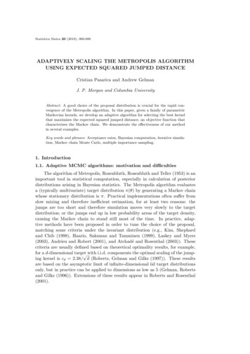
6.3 Basic Metropolis–Hastings algorithms173Fig. 6.1. Sequence X (t) for t 4500, . . . , 4800, when simulated from theMetropolis–Hastings algorithm with uniform proposal and Be(2.7, 6.3) target.Yt ’s are rejected. Note that those multiple occurrences of the same numerical valuemust be kept in the sample as such; otherwise, the validity of the approximationof f is lost! Indeed, when considering the entire chain as a sample, its histogramproperly approximates the Be(2.7, 6.3) target. Figure 6.2 shows histograms andoverlaid densities both for this Metropolis–Hastings sample and for an (exact) iidsample drawn using the rbeta command. The fits are quite similar, and this canbe checked even further using a Kolmogorov–Smirnov test of equality betweenthe two samples: ks.test(jitter(X),rbeta(5000,a,b))Two-sample Kolmogorov-Smirnov testdata: jitter(X) and rbeta(5000,a,b)D 0.0202, p-value 0.2594alternative hypothesis: two-sidedwhich states that both samples are compatible with the same distribution. Anadditional (if mild) check of agreement is provided by the moments. For instance,since the mean and variance of a Be(a, b) distribution are a/(a b) and ab/(a b)2 (a b 1), respectively, we can compareX̄ .301 ,S 2 .0205 ,with the theoretical values of .3 for the mean and .021 for the variance.JWhile the MCMC and exact sampling outcomes look identical in Figure6.2, it is important to remember that the Markov chain Monte Carlo samplehas correlation, while the iid sample does not. This means that the qualityof the sample is necessarily degraded or, in other words, that we need more
1746 Metropolis–Hastings AlgorithmsFig. 6.2. Histograms of beta Be(2.7, 6.3) random variables with density function overlaid. In the left panel, the variables were generated from a Metropolis–Hastings algorithm with a uniform candidate, and in the right panel the randomvariables were directly generated using rbeta(n,2.7,6.3).simulations to achieve the same precision. This issue is formalized throughthe notion of effective sample size for Markov chains (Section 8.4.3).In the symmetric case (that is, when q(x y) q(y x)), the acceptance probability ρ(xt , yt ) is driven by the objective ratio f (yt )/f (x(t) ) and thus even theacceptance probability is independent from q. (This special case is detailed inSection 6.4.1.) Again, Metropolis–Hastings algorithms share the same featureas the stochastic optimization Algorithm 2 (see Section 5.5), namely that theyalways accept values of yt such that the ratio f (yt )/q(yt x(t) ) is increased compared with the “previous” value f (x(t) )/q(x(t) yt ). Some values yt such thatthe ratio is decreased may also be accepted, depending on the ratio of the
6.3 Basic Metropolis–Hastings algorithms175ratios, but if the decrease is too sharp, the proposed value yt will almost always be rejected. This property indicates how the choice of q can impact theperformance of the Metropolis–Hastings algorithm. If the domain explored byq (its support) is too small, compared with the range of f , the Markov chainwill have difficulties in exploring this range and thus will converge very slowly(if at all for practical purposes).Another interesting property of the Metropolis–Hastings algorithm thatadds to its appeal is that it only depends on the ratiosf (yt )/f (x(t) )andq(x(t) yt )/q(yt x(t) ) .It is therefore independent of normalizing constants. Moreover, since all thatmatters is the ability to (a) simulate from q and (b) compute the ratiof (yt )/q(yt x(t) ), q may be chosen in such a way that the intractable partsof f are eliminated in the ratio. Since q(y x) is a conditional density, it integrates to one in y and, assuch, involves a functional term that depends on both y and x as wellas a normalizing term that depends on x, namely q(y x) C(x)q̃(x, y).When noting above that the Metropolis–Hastings acceptance probabilitydoes not depend on normalizing constants, terms like C(x) are obviouslyexcluded from this remark since they must appear in the acceptance probability, lest it jeopardize the stationary distribution of the chain.6.3.2 The independent Metropolis–Hastings algorithmThe Metropolis–Hastings algorithm of Section 6.3.1 allows a candidate distribution q that only depends on the present state of the chain. If we now requirethe candidate q to be independent of this present state of the chain (that is,q(y x) g(y)), we do get a special case of the original algorithm:Algorithm 5 Independent Metropolis–HastingsGiven x(t)1. Generate Yt g(y).2. Take f (Yt ) g(x(t) ) Ywith probability min,1tX (t 1) f (x(t) ) g(Yt ) (t)xotherwise.
1766 Metropolis–Hastings AlgorithmsThis method then appears as a straightforward generalization of theAccept–Reject method in the sense that the instrumental distribution is thesame density g as in the Accept–Reject method. Thus, the proposed valuesYt are the same, if not the accepted ones.Metropolis–Hastings algorithms and Accept–Reject methods (Section 2.3),both being generic simulation methods, have similarities between them thatallow comparison, even though it is rather rare to consider using a Metropolis–Hastings solution when an Accept–Reject algorithm is available. In particular,consider thata. The Accept–Reject sample is iid, while the Metropolis–Hastings sample isnot. Although the Yt ’s are generated independently, the resulting sampleis not iid, if only because the probability of acceptance of Yt depends onX (t) (except in the trivial case when f g).b. The Metropolis–Hastings sample will involve repeated occurrences of thesame value since rejection of Yt leads to repetition of X (t) at time t 1.This will have an impact on tests like ks.test that do not accept ties.c. The Accept–Reject acceptance step requires the calculation of the upperbound M supx f (x)/g(x), which is not required by the Metropolis–Hastings algorithm. This is an appealing feature of Metropolis–Hastings ifcomputing M is time-consuming or if the existing M is inaccurate andthus induces a waste of simulations.Exercise 6.3 Compute the acceptance probability ρ(x, y) in the case q(y x) g(y). Deduce that, for a given value x(t) , the Metropolis–Hastings algorithmassociated with the same pair (f, g) as an Accept–Reject algorithm accepts theproposed value Yt more often than the Accept–Reject algorithm.The following exercise gives a first comparison of Metropolis–Hastings withan Accept–Reject algorithm already used in Exercise 2.20 when both algorithms are based on the same candidate.Exercise 6.4 Consider the target as the G(α, β) distribution and the candidateas the gamma G([α], b) distribution (where [a] denotes the integer part of a).a. Derive the corresponding Accept–Reject method and show that, when β 1,the optimal choice of b is b [α]/α.b. Generate 5000 G(4, 4/4.85) random variables to derive a G(4.85, 1) sample(note that you will get less than 5000 random variables).c. Use the same sample in the corresponding Metropolis–Hastings algorithm togenerate 5000 G(4.85, 1) random variables.d. Compare the algorithms using (i) their acceptance rates and (ii) the estimatesof the mean and variance of the G(4.85, 1) along with their errors. (Hint:Examine the correlation in both samples.)
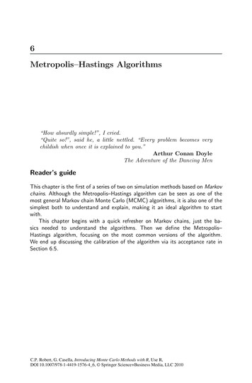
6.3 Basic Metropolis–Hastings algorithms177Fig. 6.3. Histograms and autocovariance functions from a gamma Accept–Reject algorithm (left panels) and a gamma Metropolis–Hastings algorithm (rightpanels). The target is a G(4.85, 1) distribution and the candidate is a G(4, 4/4.85)distribution. The autocovariance function is calculated with the R function acf.Figure 6.3 illustrates Exercise 6.4 by comparing both Accept–Reject andMetropolis–Hastings samples. In this setting, operationally, the independent Metropolis–Hastings algorithm performs very similarly to the Accept–Reject algorithm, which in fact generates perfect and independent randomvariables.Theoretically, it is also feasible to use a pair (f, g) such that a bound M onf /g does not exist and thus to use Metropolis–Hastings when Accept–Reject isnot possible. However, as detailed in Robert and Casella (2004) and illustrated in the following formal example, the performance of the Metropolis–Hastings algorithm is then very poor, while it is very strong as long assup f /g M .
1786 Metropolis–Hastings AlgorithmsExample 6.2. To generate a Cauchy random variable (that is, when f corresponds to a C(0, 1) density), formally it is possible to use a N (0, 1) candidatewithin a Metropolis–Hastings algorithm. The following R code will do it: Nsim 10 4 X c(rt(1,1))# initialize the chain from the stationary for (t in 2:Nsim){ Y rnorm(1)# candidate normal rho dt(Y,1)*dnorm(X[t-1])/(dt(X[t-1],1)*dnorm(Y)) X[t] X[t-1] (Y-X[t-1])*(runif(1) rho) }When executing this code, you may sometimes start with a large value for X (0) ,12.788 say. In this case, dnorm(X[t-1]) is equal to 0 because, while 12.788can formally be a realization from a normal N (0, 1), it induces computationalunderflow problems pnorm(12.78,log T,low F)/log(10)[1] -36.97455(meaning the probability of exceeding 12.78 is 10 37 ) and the Markov chainremains constant for the 104 iterations! If the chain starts from a more centralvalue, the outcome will resemble a normal sample much more than a Cauchysample, as shown by Figure 6.4 (center right). In addition, very large values ofthe sequence will be heavily weighted, resulting in long strings where the chainremains constant, as shown by Figure 6.4, the isolated peak in the histogrambeing representative of such an occurrence. If instead we use for the independentproposal g a Student’s t distribution with .5 degrees of freedom (that is, if wereplace Y rnorm(1) with Y rt(1,.5) in the code above), the behavior of thechain is quite different. Very large values of Yt may occur from time to time (asshown in Figure 6.4 (upper left)), the histogram fit is quite good (center left),and the sequence exhibits no visible correlation (lower left). If we consider theapproximation of a quantity like Pr(X 3), for which the exact value is pt(3,1)(that is, 0.896), the difference between the two choices of g is crystal clear inFigure 6.5, obtained by plot(cumsum(X 3)/(1:Nsim),lwd 2,ty "l",ylim c(.85,1)).The chain based on the normal proposal is consistently off the true value, whilethe chain based on the t distribution with .5 degrees of freedom converges quitequickly to this value. Note that, from a theoretical point of view, the Metropolis–Hastings algorithm associated with the normal proposal still converges, but theconvergence is so slow as to be useless.JWe now look at a somewhat more realistic statistical example that corresponds to the general setting when an independent proposal is derived froma preliminary estimation of the parameters of the model. For instance, whensimulating from a posterior distribution π(θ x) π(θ)f (x θ), this independent
6.3 Basic Metropolis–Hastings algorithms179Fig. 6.4. Comparison of two Metropolis–Hastings schemes for a Cauchy targetwhen generating (left) from a N (0, 1) proposal and (right) from a T1/2 proposalbased on 105 simulations. (top) Excerpt from the chains (X (t) ); (center) histogramsof the samples; (bottom) autocorrelation graphs obtained by acf.proposal could be a normal or a t distribution centered at the MLE θ̂ and withvariance-covariance matrix equal to the inverse of Fisher’s information matrix.Example 6.3. The cars dataset relates braking distance (y) to speed (x) in asample of cars. Figure 6.6 shows the data along with a fitted quadratic curve thatis given by the R function lm. The model posited for this dataset is a quadraticmodelyij a bxi cx2i εij , i 1, . . . , k, j 1, . . . ni ,where we assume that εij N (0, σ 2 ) and independent. The likelihood functionis then proportional to
1806 Metropolis–Hastings AlgorithmsFig. 6.5. Example 6.2: cumulative coverage plot of a Cauchy sequence generatedby a Metropolis–Hastings algorithm based on a N (0, 1) proposal (upper lines) andone generated by a Metropolis–Hastings algorithm based on a T1/2 proposal (lowerlines). After 105 iterations, the Metropolis–Hastings algorithm based on the normalproposal has not yet converged. 1σ2 N/2 1 X 2 2exp(y a bx cx),ijii 2σ 2 ijPwhere N i ni is the total number of observations. We can view this likelihoodfunction as a posterior distribution on a, b, c, and σ 2 (for instance based on a flatprior), and, as a toy problem, we can try to sample from this distribution with aMetropolis–Hastings algorithm (since this standard distribution can be simulateddirectly; see Exercise 6.12). To start with, we can get a candidate by generatingcoefficients according to their fitted sampling distribution. That is, we can usethe R command x2 x 2 summary(lm(y x x2))to get the output
6.3 Basic Metropolis–Hastings algorithms181Fig. 6.6. Braking data with quadratic curve (dark) fitted with the least squaresfunction lm. The grey curves represent the Monte Carlo sample (a(i) , b(i) , c(i) ) andshow the variability in the fitted lines based on the last 500 iterations of 4000simulations.Coefficients:Estimate Std. Error(Intercept) 2.63328 14.80693x0.88770 2.03282x20.10068 0.06592Residual standard error: 15.17 ont value Pr( t )0.178 0.8600.437 0.6641.527 0.13347 degrees of freedomAs suggested above, we can use the candidate normal distribution centered at theMLEs,a N (2.63, (14.8)2 ),b N (.887, (2.03)2 ),c N (.100, (0.065)2 ),σ 2 G(n/2, (n 3)(15.17)2 ),in a Metropolis–Hastings algorithm to generate samples (a(i) , b(i) , c(i) ). Figure6.6 illustrates the variability of the curves associated with the outcome of thissimulation.J
1826 Metropolis–Hastings Algorithms6.4 A selection of candidatesThe study of independent Metropolis–Hastings algorithms is certainly interesting, but their practical implementation is more problematic in that theyare delicate to use in complex settings because the construction of the proposal is complicated—if we are using simulation, it is often because derivingestimates like MLEs is difficult—and because the choice of the proposal ishighly influential on the performance of the algorithm. Rather than buildinga proposal from scratch or suggesting a non-parametric approximation basedon a preliminary run—because it is unlikely to work for moderate to highdimensions—it is therefore more realistic to gather information about thetarget stepwise, that is, by exploring the neighborhood of the current valueof the chain. If the exploration mechanism has enough energy to reach as faras the boundaries of the support of the target f , the method will eventuallyuncover the complexity of the target. (This is fundamentally the same intuition at work in the simulated annealing algorithm of Section 5.3.3 and thestochastic gradient method of Section 5.3.2.)6.4.1 Random walksA more natural approach for the practical construction of a Metropolis–Hastings proposal is thus to take into account the value previously simulatedto generate the following value; that is, to consider a local exploration of theneighborhood of the current value of the Markov chain.The implementation of this idea is to simulate Yt according toYt X (t) εt ,where εt is a random perturbation with distribution g independent of X (t) ,for instance a uniform distribution or a normal distribution, meaning thatYt U(X (t) δ, X (t) δ) or Yt N (X (t) , τ 2 ) in unidimensional settings.In terms of the general Metropolis–Hastings algorithm, the proposal densityq(y x) is now of the form g(y x). The Markov chain associated with q isa random walk (as described in Section 6.2) when the density g is symmetric around zero; that is, satisfying g( t) g(t). But, due to the additionalMetropolis–Hastings acceptance step, the Metropolis–Hastings Markov chain{X (t) } is not a random walk. This approach leads to the following Metropolis–Hastings algorithm, which also happens to be the original one proposed byMetropolis et al. (1953).Algorithm 6 Random walk Metropolis–HastingsGiven x(t) ,1. Generate Yt g(y x(t) ).
6.4 A selection of candidates1832. TakeX(t 1) (Ytx(t)no with probability min 1, f (Yt ) f (x(t) ) ,otherwise.As noted above, the acceptance probability does not depend on g. Thismeans that, for a given pair (x(t) , yt ), the probability of acceptance is thesame whether yt is generated from a normal or from a Cauchy distribution.Obviously, changing g will result in different ranges of values for the Yt ’s anda different acceptance rate, so this is not to say that the choice of g has noimpact whatsoever on the behavior of the algorithm, but this invariance ofthe acceptance probability is worth noting. It is actually linked to the factthat, for any (symmetric) density g, the invariant measure associated withthe random walk is the Lebesgue measure on the corresponding space (seeMeyn and Tweedie, 1993).Example 6.4. The historical example of Hastings (1970) considers the formalproblem of generating the normal distribution N (0, 1) based on a random walkproposal eq
The Metropolis{Hastings algorithm is an example of those methods. (Gibbs sampling, described in Chapter 7, is another example with equally uni-versal potential.) Given the target density f, it is associated with a working conditional density q(yjx) that, in practice, is easy to simulate. In addition, q