Transcription
Chapter 4 – MicroscopyGabriel PopescuUniversityy of Illinois at Urbana‐Champaignp gBeckman InstituteQuantitative Light Imaging Laboratoryhttp://light.ece.uiuc.eduPrinciples of Optical ImagingElectrical and Computer Engineering, UIUC
ECE 460 – Optical Imaging4.1 Resolution of Optical Microscopes The Microscopep can be approximatedppbyy 2 lenses F [ F [U [ x , y ]]]SampleTube lensObjectiveF2F2’F’’1U(x,y)F1[U [ x, y ]]F2 [ F1[U [ x, y ]]] U [ x y , ]M M “‐” sign means inverted image The objective is the most important part of the microscope Usually a third lens (ocular) images F2’ at , such that we canvisualize it with the relaxed eye.Chapter 4: Microscopy2
ECE 460 – Optical Imaging4.1 Resolution of Optical Microscopes The objectivejlens dictates the resolution or size of thesmallest object that the microscope can resolve. Contrast is generated by absorption, scattering, etc. Microscopes can be categorized by the methods that they useto produce contrast. LetLet’ss consider an infinitely small object (point):x1x2xMθfChapter 4: MicroscopyHow small can we see?f3
ECE 460 – Optical Imaging4.1 Resolution of Optical Microscopes Fourier ppropertiespof the lens;; the reconstructed field is: U [ x, y ] U[, ]e2 i ( x1ξ y1 )d d (4.1) xξ M fM and yM f We know that ξ and because We can access only a finite frequency range and therefore wecan only achieve finite resolution. We would need an infinite spectrum to reconstruct ad‐function (in this case a point)MChapter 4: Microscopy4
ECE 460 – Optical Imaging4.1 Resolution of Optical Microscopes Given the finite frequencyqy supportpp we can write:U [ , ] U [ , ] H [ , ] WhereH {1 if ξ ξ M , 0 o th e rw is e1ξ(4.2)Mξξξ So, eq. 4.1 becomesU [ x, y ] F [U [ , ] H [ , ]]Chapter 4: Microscopy(4.3)5
ECE 460 – Optical Imaging4.1 Resolution of Optical Microscopes Use the Convolution Theorem once more ((which states thatconvolution in one domain is multiplication in another) to get:U [ x, y ] U [ x, y ] V h[ x, y ] Where U [ x, y ] is the microscope imageU [ x, y ] is the ideal imageh[ x, y ] is the impulse responseeh[ x, y ] F [ H [ , ]] H[ fx , f y ] Chapter 4: Microscopy 1 if f x 2 f y 2 w20 otherwise i ( x ξ y )(4.4)(4.5)pL circ[ ] w(4.6)2w6
ECE 460 – Optical Imaging4.1 Resolution of Optical MicroscopesF [H ] A J 1[ 2 W ] h,2 W w h e re J is a B e sse l fu n c tio n o f th e 1 st k in d a n d o rd e r So,, So the image of a “point” becomes:h[ x , y ] Since WM xM f 2A2 1J 1[2 W ]2 W and 2W M 1 .2 2 .6161 fxM(eq. 4.8)(4.7)2xM2 1.22 f so,so2J1[ x] x The Airy Function‐1.221.22 A point will be imaged as a smeared spot of diameter .61Chapter 4: MicroscopyxH fxM7
ECE 460 – Optical Imaging4.1 Resolution of Optical Microscopes Imagineg that we have two such points.pThen the resolution isthe minimum distance between the points that are separated,ρwhich is ρ. resolution An objectivejlens that allows highergspatialpfrequenciesq((orangles) provides a higher resolution.Chapter 4: Microscopy8
ECE 460 – Optical Imaging4.1 Resolution of Optical MicroscopesxM 1 1Sx2Ob2x1Ob1xM 2 2Sf1f1xMsin tan Definition:11ff2f2sin 1 NA Numerical Aperture TheTh resolutionl i becomesbbbut .61NA Compare Ob1 and Ob2 above: 2NA(4.10)iis goodd enoughh 1 2 , xM 1 xM 2 NA1 NA2 1 2(4 11)(4.11) So Ob2 provides a better resolution.Chapter 4: Microscopy9
ECE 460 – Optical Imaging4.1 Resolution of Optical Microscopes In general, objectives are made out of several lenses complex systemsPP'FWfEntrance PupilObjectivejf focal distance measured from principal planeW working distance distance from F to physical surface of lensEntrance Pupil image of physical aperture f and entrance pupil determine numerical aperture i.e. resolutionChapter 4: Microscopy10
ECE 460 – Optical Imaging4.1 Resolution of Optical Microscopes Note: if the objectivejlens is immersed in a medium for whichn 1, thenNA n NA (4.12)n This means that it is possible for immersed objective lenses tohave a better resolution.Chapter 4: Microscopy11
ECE 460 – Optical Imaging4.2 Contrast The final imageg consists of a distribution I [ x, y ] which is theresult of absorption, scattering/diffraction, etc. Contrast a measure of the intensity fluctuations across theiimage.I general,l thInthe more contrastt t theth bbetter.ttLow ContrastHigh ContrastIIxChapter 4: Microscopyxdemo available12
ECE 460 – Optical Imaging4.2 Contrast Microscopep imageg2 regions of interest: A, BN is the background noise (in sample)Contrast :(4.13)C AB S A S B ; S A, B signal A, B Contrast to noise ratio:CNR AB C AB N S A SB N N standard deviation of noise. ( S i S ) ; S i signal in pixels22NiChapter 4: Microscopy13
ECE 460 – Optical Imaging4.2 Contrast While resolution is ggiven byy the instrument,, the contrast isgiven by the instrument/sample combination. Most biological structures (i.e. cells) are very transparent soI [ x, y ]is flat, which means there is low contrastThey can be assumed “phase objects”Wave frontI [ x, y ]Example of a phase object:100 nmkImagingsystemN 1.5‐Glass Profile‐Phase GratingChapter 4: Microscopy14
ECE 460 – Optical Imaging4.2 Contrast No absorptionpso I [ x, y ] constant contrast 0 BUT: the wave front carries information about the sampleE[ x, y ] E0 ei [ x , y ]((4.14)) This is the expression for the field in the vicinity of a phaseobjectobject. Bright Field microscopy produces low contrast images ofphase objectspjChapter 4: Microscopy15
ECE 460 – Optical Imaging4.2 Contrast There are several ways to enhance contrast: EndogeneousgContrast Dark fieldPhase contrastSchlereinQuantitative phase microscopyConfocalgflorescenceEndogeneous Exogeneous Contrast Agents StainingFull field Florescent taggingConfocal More recently Beads (dielectric and metallic) Nano Quantum DotsChapter 4: Microscopy16
ECE 460 – Optical Imaging4.3 Dark Field Microscopy Consider the low contrast imageI( )I(x)I(x,y)x Typical low pass filtering remove CI(x)FourierI(fx)xRemove lowFrequencyfx Then take the inverse Fourier TransformationInverseFourierChapter 4: MicroscopyI(x)HighContrastx17
ECE 460 – Optical Imaging4.3 Dark Field Microscopy Actual MicroscopeObjectfLensBlocks lowfrequencyEnhanced Contrast High frequency components areenhanced ((eg.g edges)g ) Without the sampleDark FieldChapter 4: Microscopy18
ECE 460 – Optical Imaging4.4 Schlerein Method Not used very often nowadaysBlocks ½spectrumFourier Image PlaneInverse FourierEnhances ContrastPhase objects can be rendered visibleEdges are enhancedRelates to Hilbert Transform.Chapter 4: Microscopy19
ECE 460 – Optical Imaging4.4 Schlieren Method Exercise: Show the following for a real signal f(x)f(x)FourierCut ½InverseF(g) spectrum Ft(g) Fourier f(x)f (x) and f (x) 1 f (x) i P f (x') dx'22 x x'HilbertTo the left:David Hilbert aGermanMathematician,recognized asone of the mostinfluential anduniversalmathematiciansof the 19th andearly 20thcenturies.Chapter 4: Microscopy20
ECE 460 – Optical Imaging4.5 Phase Contrast Microscopy Developed by Frits Zernike (1935) yielding Noble prize in1953(Physics) Very powerful, commonly used today. Consider a phase object:U ( x, y ) ei ( x , y )(4.15) Intensity distribution:I ( x, y ) U2 1 No Contrast Assume: The microscope has a magnification M 1(x,y)SChapter 4: Microscopy(x’,y’)Fourier PlaneImageplane21
ECE 460 – Optical Imaging4.5 Phase Contrast Microscopy i 2 ( f x f y )U ( f x , f y ) U ( x, y )edxdy(4.16) fx xy; fx f f(4.17) Note: U (0, 0) U ( x, y )dxdy Central Ordinate Theorem Zero Frequency component corresponds to a plane wave inPlane Wavethe image plane(constant of (x,y)) U(x, y)dxdyChapter 4: MicroscopyU0 1U(x, y)dxdy A22
ECE 460 – Optical Imaging4.5 Phase Contrast Microscopy Note: U hash no informationi fi aboutbtheh structure off theh sample.l0U0 1U(x, y )dxdy Average field AImage formation is an interference between the average fieldand high frequency components.U( x, y ) U0 [U( x, y ) U0 ]High FrequencyCComponenttChapter 4: Microscopy(4.18)U1(x, y )23
ECE 460 – Optical Imaging4.5 Phase Contrast Microscopy Phase contrast relies on shifting the phase of U 0 byU 0 U 0 aei Assume U 0 1 ; U 0 U 0 aei becomes: U ( x, y ) aei [U ( x, y ) 1] The intensity distribution in the image plane(4 19)(4.19)becomes:2I ( x, y ) U ( x, y ) i ae ei ( x , y )2 1 a 2 1 1 Re[2[ aei ( ) 2aei 2ei ] a 2 2[1 a cos cos a cos( )]Chapter 4: Microscopy(4.20)24
ECE 460 – Optical Imaging4.5 Phase Contrast Microscopy Note: For a 0 recover Dark Field Microscopy Assume “small”small phase shift cos 1; 2I ( x , y ) a 2 2 a sin sin a 2 2 a ( x , y ) sin I ( x, y ) a 2 2a ( x, y )(4.21) PC couples into intensity a 1 enhances contrast (best modulation for U 0 U1 )Chapter 4: Microscopy25
ECE 460 – Optical Imaging4.6 Nomarski/Differential Interference ContrastMicroscopyi DIC Differential Interference n Prism #110Obj.Wollaston Prism #2 Use polarization discrimination to create 2 interferingbeamsp ( ) with 2 drifted beams Illuminate sample(s)Chapter 4: Microscopy26
ECE 460 – Optical Imaging4.6 Nomarski/Differential Interference ContrastMicroscopyi “Shift” amount Airy disk 2NA Wollaston prism #2 brings the 2 beams together throughi t finterference.ETotal E1 E0 A1 ei 1 A0 ei 0(4.22)l. lddl.d 1 0 n1k n0 d kcos Chapter 4: Microscopy27
ECE 460 – Optical Imaging4.6 Nomarski/Differential Interference ContrastMicroscopyi By varying the position of Wollaston prismone can adjust 1 0 Phase Shift through the sample:ldxxei ( x dx ).ze i ( x )S becomes:ETotal An ei ( n ) A0 ei 0 A0 ei 0 [[1 ei ( 11 0 ) ]Chapter 4: Microscopy(4.23)28
ECE 460 – Optical Imaging4.6 Nomarski/Differential Interference ContrastMicroscopyi The Intensity in the image plane (as a function ofdisplacement x).I ( x) 2I0 (1 cos[ ( x dx) ( x) ]) Note: For small , best results obtained forf (4.24) 2I ( x) 2 I 0 (1 sin[ ( x dx) ( x)]) 2 I 0 [1 dx ( x dx) ( x)](4.25)dx SoS theh finalfi l iintensityi distributiondi ib i isi relatedl d to theh gradientdiof the phase: (x) xChapter 4: Microscopy29
ECE 460 – Optical Imaging4.6 Nomarski/Differential Interference ContrastMicroscopyi DIC is a very sensitive to edges, even though the actualphase shifts are “small”. Example:samplexIIntensityt it nocontrastxx PhasePhcontrastt t andd DIC heavilyh il usedd today,t d especiallyi ll forfinvestigating live biological structures (cells) noninvasively.Chapter 4: Microscopy30
ECE 460 – Optical Imaging4.7 Quantitative Phase Microscopy PC &DIC are great, but qualitative in terms of phase ( x, y ) quantitatively KnowingKii i l offersff some advantages,di.e.igives a map of structure density; for homogeneous structures,gives molecular information. QPM is a “rather new” domain; several methods so far. Main obstacle is noiseChapter 4: Microscopy31
ECE 460 – Optical Imaging4.8 Confocal Microscopy So far, we discussed full‐ field imaging, i.e obtaining theentire image at once(great feature: imaging as a parallelprocess). The image can be recorded point by point also(like TV),sometimes with some advantages. Confocal same focal point for illumination and collectionPinholeChapter 4: Microscopy32
ECE 460 – Optical Imaging4.8 Confocal Microscopy Due to pinhole, light out of focus is rejected, which cancreate stacks of slicesslices, hence 3D rendering Scanning: either by scanning the sample or the beam Note: 3D Info large field of view (limited by aperture) up to 2 better resolutionBS ! It works in reflection usuallyPinholeChapter 4: Microscopy33
ECE 460 – Optical Imaging4.8 Confocal Microscopy/ NSOM Recent development: Multi Foci ImprovesIacquisitioni i i timei Need more power Trade‐offMultipleFocused beam Confocal can provide many frames/seconds(video rate) Leading to 4D imaging(x,y,z,t)Chapter 4: Microscopy34
ECE 460 – Optical Imaging4.8 Confocal Microscopy/ NSOM Near Field Scanning Optical Microscope(NSOM) ContinuationC ii off confocalf l & AFM Tappered fiber as cantilever :FiberAperture down to 50 nmEvanescent waves(no transmission in air)Chapter 4: Microscopy35
ECE 460 – Optical Imaging4.8 Confocal Microscopy/ NSOMSample 50 100nmD Evanescent waves couple into sample Became propagating Not limitedldbby diffractiond ff Drawback: scanning time; difficult in liquidsChapter 4: Microscopy36
ECE 460 – Optical Imaging4.9 Fluorescence Microscopy Illumination and emission have different wavelengthsEndogenous “Fluorophoress” eg. NADHMost commonly exogenousRecently: GFP technology (given fluorescent protein) genetically encodedencoded, fused with DNA GFP live cell imagingfluorophores allows for multiple “fluorophores” dynamic monitoring of processes(cell signaling)Chapter 4: Microscopy37
ECE 460 – Optical Imaging4.9 Fluorescence Microscopy Fluorescence adds specificity to the measurement.(organelle dynamicsdynamics, process specific) Typically‐ epi‐fluorescence( reflection geometry)SObj.BS Filter Filter blocks the excitation lightChapter 4: Microscopy38
ECE 460 – Optical Imaging4.9 Fluorescence Microscopy Full‐Field is limited to thin samples Combine fluorescence & confocal leads to deeper penetration Issues when imaging live cells: acquisition time, sensitivity, damage. Photo‐bleaching can produce cell damage: limit duration of illumination need efficiency sensitivity use intensifiediifi d CCD Acquisition speed: improve with multi‐foci &Nipkow disk scanningChapter 4: Microscopy39
ECE 460 – Optical Imaging4.9 Fluorescence Microscopy Other Fluorescence Techniques: TotalT l iinternall reflectionfl i FCS‐Fluorescence correlation spectroscopy FRAP‐Fluorescence recovery after photobleaching FRET‐Fluorescence resonance energy transfer. FLIM‐fluorescence lifetime imaging.g g STED‐Stimulated emission depletion 100nm spot STED 4Pi confocal microscopy 33nm diffraction spotsingle molecule imaging. PALM, fPALM Fiona,Fiona etcChapter 4: Microscopy40
ECE 460 – Optical Imaging4.10 Multiphoton Imaging 2‐ Photon laser scanning microscopyN liNonlinearprocessDeep PenetrationRequires high power densityI f I 2x1Improves ResolutionIllumination spotp isreduce by2z0Fluorescence Chapter 4: Microscopy41
ECE 460 – Optical Imaging4.10 Multiphoton Imaging 2nd harmonic Imaging‐recent:E dEndogenousSHG molecules(e.gl l ( collagen)ll)P (L) E2 coherent process (phase matching)Same advantage of smaller illumination spotLet’s take a look at examples!Chapter 4: Microscopy42
Microscopy imageshttp://www.microscopyu.com/Nikon
1. Cell imaging
ikon
2. Tissue slice imaging
Confocal fluorescence
Chapter 4 -Microscopy Gabriel Popescu University of Illinois at Urbana‐Champpgaign Beckman Institute Quantitative LightImaging Laboratory Principles of Optical Imaging Electrical and Computer Engineering, UIUC