Transcription
The Shallow Water EquationsClint Dawson and Christopher M. MirabitoInstitute for Computational Engineering and SciencesUniversity of Texas at Austinclint@ices.utexas.eduSeptember 29, 2008
IntroductionDerivation of the SWEThe Shallow Water Equations (SWE)What are they?The SWE are a system of hyperbolic/parabolic PDEs governing fluidflow in the oceans (sometimes), coastal regions (usually), estuaries(almost always), rivers and channels (almost always).The general characteristic of shallow water flows is that the verticaldimension is much smaller than the typical horizontal scale. In thiscase we can average over the depth to get rid of the verticaldimension.The SWE can be used to predict tides, storm surge levels andcoastline changes from hurricanes, ocean currents, and to studydredging feasibility.SWE also arise in atmospheric flows and debris flows.C. MirabitoThe Shallow Water Equations
IntroductionDerivation of the SWEThe SWE (Cont.)How do they arise?The SWE are derived from the Navier-Stokes equations, whichdescribe the motion of fluids.The Navier-Stokes equations are themselves derived from theequations for conservation of mass and linear momentum.C. MirabitoThe Shallow Water Equations
IntroductionDerivation of the SWEDerivation of the Navier-Stokes EquationsBoundary ConditionsSWE Derivation ProcedureThere are 4 basic steps:1Derive the Navier-Stokes equations from the conservation laws.2Ensemble average the Navier-Stokes equations to account for theturbulent nature of ocean flow. See [1, 3, 4] for details.3Specify boundary conditions for the Navier-Stokes equations for awater column.4Use the BCs to integrate the Navier-Stokes equations over depth.In our derivation, we follow the presentation given in [1] closely, but wealso use ideas in [2].C. MirabitoThe Shallow Water Equations
IntroductionDerivation of the SWEDerivation of the Navier-Stokes EquationsBoundary ConditionsConservation of MassConsider mass balance over a control volume Ω. ThenZZdρ dV (ρv) · n dA,dt Ω {z} Ω {z}Time rate of changeof total mass in ΩNet mass flux acrossboundary of Ωwhereρ is the fluid density (kg/m3 ), uv v is the fluid velocity (m/s), andwn is the outward unit normal vector on Ω.C. MirabitoThe Shallow Water Equations
IntroductionDerivation of the SWEDerivation of the Navier-Stokes EquationsBoundary ConditionsConservation of Mass: Differential FormApplying Gauss’s Theorem givesZZdρ dV · (ρv) dV .dt ΩΩAssuming that ρ is smooth, we can apply the Leibniz integral rule: Z ρ · (ρv) dV 0.Ω tSince Ω is arbitrary, ρ · (ρv) 0 tC. MirabitoThe Shallow Water Equations
IntroductionDerivation of the SWEDerivation of the Navier-Stokes EquationsBoundary ConditionsConservation of Linear MomentumNext, consider linear momentum balance over a control volume Ω. ThenZZZZdρv dV (ρv)v · n dA ρb dV Tn dA,dt Ω{z} Ω {z} Ω{z} Ω{z}Time rate ofchange of totalmomentum in ΩNet momentum fluxacross boundary of ΩBody forcesacting on ΩExternal contactforces actingon Ωwhereb is the body force density per unit mass acting on the fluid (N/kg),andT is the Cauchy stress tensor (N/m2 ). See [5, 6] for more detailsand an existence proof.C. MirabitoThe Shallow Water Equations
IntroductionDerivation of the SWEDerivation of the Navier-Stokes EquationsBoundary ConditionsConservation of Linear Momentum: Differential FormApplying Gauss’s Theorem again (and rearranging) givesZZZZdρv dV · (ρvv) dV ρb dV · T dV 0.dt ΩΩΩΩAssuming ρv is smooth, we apply the Leibniz integral rule again: Z (ρv) · (ρvv) ρb · T dV 0.Ω tSince Ω is arbitrary, (ρv) · (ρvv) ρb · T 0 tC. MirabitoThe Shallow Water Equations
IntroductionDerivation of the SWEDerivation of the Navier-Stokes EquationsBoundary ConditionsConservation Laws: Differential FormCombining the differential forms of the equations for conservation ofmass and linear momentum, we have: ρ · (ρv) 0 t (ρv) · (ρvv) ρb · T tTo obtain the Navier-Stokes equations from these, we need to make someassumptions about our fluid (sea water), about the density ρ, and aboutthe body forces b and stress tensor T.C. MirabitoThe Shallow Water Equations
IntroductionDerivation of the SWEDerivation of the Navier-Stokes EquationsBoundary ConditionsSea water: Properties and AssumptionsIt is incompressible. This means that ρ does not depend on p. Itdoes not necessarily mean that ρ is constant! In ocean modeling, ρdepends on the salinity and temperature of the sea water.Salinity and temperature are assumed to be constant throughout ourdomain, so we can just take ρ as a constant. So we can simplify theequations: · v 0, ρv · (ρvv) ρb · T. tSea water is a Newtonian fluid. This affects the form of T.C. MirabitoThe Shallow Water Equations
IntroductionDerivation of the SWEDerivation of the Navier-Stokes EquationsBoundary ConditionsBody Forces and Stresses in the Momentum EquationWe know that gravity is one body force, soρb ρg ρbothers ,whereg is the acceleration due to gravity (m/s2 ), andbothers are other body forces (e.g. the Coriolis force in rotatingreference frames) (N/kg). We will neglect for now.For a Newtonian fluid,T pI T̄where p is the pressure (Pa) and T̄ is a matrix of stress terms.C. MirabitoThe Shallow Water Equations
IntroductionDerivation of the SWEDerivation of the Navier-Stokes EquationsBoundary ConditionsThe Navier-Stokes EquationsSo our final form of the Navier-Stokes equations in 3D are: · v 0, ρv · (ρvv) p ρg · T̄, tC. MirabitoThe Shallow Water Equations
IntroductionDerivation of the SWEDerivation of the Navier-Stokes EquationsBoundary ConditionsThe Navier-Stokes EquationsWritten out: u v w 0 x y z(1) (τxx p) τxy τxz (ρu) (ρu 2 ) (ρuv ) (ρuw ) t x y z x y z(2) (ρv ) (ρuv ) (ρv 2 ) (ρvw ) τx y (τyy p) τyz t x y z x y z(3) (ρw ) (ρuw ) (ρvw ) (ρw 2 ) τxz τyz (τzz p) ρg t x y z x y z(4)C. MirabitoThe Shallow Water Equations
IntroductionDerivation of the SWEDerivation of the Navier-Stokes EquationsBoundary ConditionsA Typical Water Columnζ ζ(t, x, y ) is the elevation (m) of the free surface relative to thegeoid.b b(x, y ) is the bathymetry (m), measured positive downwardfrom the geoid.H H(t, x, y ) is the total depth (m) of the water column. Notethat H ζ b.C. MirabitoThe Shallow Water Equations
IntroductionDerivation of the SWEDerivation of the Navier-Stokes EquationsBoundary ConditionsA Typical Bathymetric ProfileBathymetry of the Atlantic Trench. Image courtesy USGS.C. MirabitoThe Shallow Water Equations
IntroductionDerivation of the SWEDerivation of the Navier-Stokes EquationsBoundary ConditionsBoundary ConditionsWe have the following BCs:1At the bottom (z b)No slip: u v 0No normal flow:u b b v w 0 x y(5)Bottom shear stress: b b τxy τxz x yis specified bottom friction (similarly for y direction).τbx τxxwhere τbx2(6)At the free surface (z ζ)No relative normal flow: ζ ζ ζ u v w 0 t x y(7)p 0 (done in [2])Surface shear stress:τsx τxx ζ ζ τxy τxz x ywhere the surface stress(e.g. wind)τsx Wateris specified(similary for yC. MirabitoThe ShallowEquations(8)
IntroductionDerivation of the SWEDerivation of the Navier-Stokes EquationsBoundary Conditionsz-momentum EquationBefore we integrate over depth, we can examine the momentum equationfor vertical velocity. By a scaling argument, all of the terms except thepressure derivative and the gravity term are small.Then the z-momentum equation collapses to p ρg zimplying thatp ρg (ζ z).This is the hydrostatic pressure distribution. Then p ζ ρg x xwith similar form for p y .C. MirabitoThe Shallow Water Equations(9)
IntroductionDerivation of the SWEDerivation of the Navier-Stokes EquationsBoundary ConditionsThe 2D SWE: Continuity EquationWe now integrate the continuity equation · v 0 from z b toz ζ. Since both b and ζ depend on t, x, and y , we apply the Leibnizintegral rule:Zζ · v dz0 bZ ζ b v u x y ζ ydz w z ζ w z bζ ζ bv dz u z ζ u z b x x b b ζ b v z ζ v z b w z ζ w z b y y xZu dz ZC. MirabitoThe Shallow Water Equations
IntroductionDerivation of the SWEDerivation of the Navier-Stokes EquationsBoundary ConditionsThe Continuity Equation (Cont.)Defining depth-averaged velocities asū 1HZζu dz, bv̄ 1HZζv dz, bwe can use our BCs to get rid of the boundary terms. So thedepth-averaged continuity equation is H (H ū) (H v̄ ) 0 t x yC. MirabitoThe Shallow Water Equations(10)
IntroductionDerivation of the SWEDerivation of the Navier-Stokes EquationsBoundary ConditionsLHS of the x- and y -Momentum EquationsIf we integrate the left-hand side of the x-momentum equation overdepth, we get:Zζ[ b 2 u u (uv ) (uw )] dz t x y z Diff. adv. (H ū) (H ū 2 ) (H ūv̄ ) terms t x y(11)The differential advection terms account for the fact that the average ofthe product of two functions is not the product of the averages.We get a similar result for the left-hand side of the y -momentumequation.C. MirabitoThe Shallow Water Equations
IntroductionDerivation of the SWEDerivation of the Navier-Stokes EquationsBoundary ConditionsRHS of x- and y -Momentum EquationsIntegrating over depth gives us( ρgH ζ x τsx τbx ζ ρgH y τsy τby x xC. MirabitoRζτxxR bζτ b xy y yRζR bζτxyτ b yyThe Shallow Water Equations(12)
IntroductionDerivation of the SWEDerivation of the Navier-Stokes EquationsBoundary ConditionsAt long last. . .Combining the depth-integrated continuity equation with the LHS andRHS of the depth-integrated x- and y -momentum equations, the 2D(nonlinear) SWE in conservative form are: H (H ū) (H v̄ ) 0 t x y ζ1 (H ū) H ū 2 (H ūv̄ ) gH [τsx τbx Fx ] t x y xρ ζ12(H v̄ ) (H ūv̄ ) H v̄ gH [τsy τby Fy ] t x y yρThe surface stress, bottom friction, and Fx and Fy must still determinedon a case-by-case basis.C. MirabitoThe Shallow Water Equations
IntroductionDerivation of the SWEDerivation of the Navier-Stokes EquationsBoundary ConditionsReferencesC. B. Vreugdenhil: Numerical Methods for Shallow Water Flow,Boston: Kluwer Academic Publishers (1994)E. J. Kubatko: Development, Implementation, and Verification ofhp-Discontinuous Galerkin Models for Shallow Water Hydrodynamicsand Transport, Ph.D. Dissertation (2005)S. B. Pope: Turbulent Flows, Cambridge University Press (2000)J. O. Hinze: Turbulence, 2nd ed., New York: McGraw-Hill (1975)J. T. Oden: A Short Course on Nonlinear Continuum Mechanics,Course Notes (2006)R. L. Panton: Incompressible Flow, Hoboken, NJ: Wiley (2005)C. MirabitoThe Shallow Water Equations
Introduction Derivation of the SWE Derivation of the Navier-Stokes Equations Boundary Conditions SWE Derivation Procedure There are 4 basic steps: 1 Derive the Navier-Stokes equations from the conservation laws. 2 Ensemble average the Navier-Stokes equations to account for the turbulent nature of ocean