WIXLIB

ˆ ϕ̂S (x̂, t) I ˆ η̂(x̂, t) and its determinant by J.ˆWe denote the deformation gradient by F̂ (x̂, t) To track the deformation of the fluid domain in time, we introduce a smooth, invertible, ALE mappingϕ̂F : Ω̂F [0, T ] ΩF (t) given byfor all x̂ Ω̂F , t [0, T ],ϕ̂F (x̂, t) x̂ η̂F (x̂, t),where η̂F denotes the fluid displacement. We assume that η̂F equals the structure displacement at thefluid-structure interface, and that it is arbitrarily extended onto the fluid domain Ω̂F [17]. To simplify thenotation, we will writeZZv n instead ofv n A(tn ) A 1 (tm )Ω(tm )Ω(tm )whenever we need to integrate v n on a domain Ω(tm ), for m 6 n.To model the fluid flow, we use the Navier-Stokes equations in the ALE formulation [35, 7, 6], given by ρF t u Ω̂F (u w) · u · σF (u, p) fFin ΩF (t) (0, T ),(2.1) ·u 0in ΩF (t) (0, T ),(2.2)where u is the fluid velocity, ρF is fluid density, σF is the Cauchy stress tensor and fF is the forcing term.For a Newtonian fluid, the Cauchy stress tensor is given by σF (u, p) pI 2µF D(u), where p is the fluidpressure, µF is the fluid viscosity and D(u) ( u ( u)T )/2 is the strain rate tensor. Notation t u Ω̂Fdenotes the Eulerian description of the ALE field t u A [22], i.e., t u(x, t) Ω̂F t u(A 1 (x, t), t),and the domain velocity is denoted by w t x Ω̂F t A A 1 .To model the elastic structure, we use the elastodynamics equations written in the first order form as ˆ · F̂ Ŝρ̂S t ξ̂ in Ω̂S (0, T ),(2.3a)in Ω̂S (0, T ), t η̂ ξ̂(2.3b)where ξ̂ and η̂ are the solid velocity and displacement, respectively, ρ̂S is the density of the solid material,and Ŝ is the second Piola-Kirchhoff stress tensor. The particular choices of Ŝ will be specified in Section 5.The Cauchy stress tensor for the elastic structure is given byσS Jˆ 1 F̂ Ŝ F̂ T .The solid velocity and displacement in the reference configuration are related to their Eulerian counterpartsvia ξ̂ ξ ϕ̂S and η̂ η ϕ̂S , respectively.To couple the fluid and structure, we prescribe the kinematic and dynamic coupling conditions. Thekinematic (no-slip) coupling condition describes the continuity of velocity at the fluid-structure interface,given byu ξ on Γ(t) (0, T ).(2.4)The dynamic coupling condition describes the continuity of stresses at the fluid-structure interface, prescribedasσF nF σS nS 0 on Γ(t) (0, T ),(2.5)where nF and nS are the outward unit normals to the boundaries of the deformed fluid and structuredomains, respectively. The fluid and structure problems are complemented with initial and boundary conditions.3

3. Numerical method. In this section, we propose a time-adaptive, partitioned numerical schemefor the fluid-structure interaction based on the strongly-coupled partitioned method developed in [10]. Thetime integration used in this work is based on the refactorized Cauchy’s one-legged ‘θ like’ method, whichis combined with the partitioned approach used in [44]. The resulting method is adaptive, strongly-coupled,unconditionally stable when θ [ 21 , 1] and second order accurate when θ 12 O(τ n ), where τ n is the timestep.The main steps in the derivation of the refactorized Cauchy’s one-legged ‘θ like’ method are summarizedas follows. Let {tn }0 n N denote mesh points based on a variable time step τn such that tn 1 tn τn .For an initial value problem y 0 f (t, y(t)), the adaptive Cauchy’s one-legged ‘θ like’ method is given asy n 1 y n f (tn θn , y n θn ),τn(3.1)for θn [0, 1], where tn θn tn θn τn and y n θn θn y n 1 (1 θn )y n . We note that this method is equalto the “classical” θ method when f is linear. However, for nonlinear problems with variable time-stepping,the Cauchy’s one-legged ‘θ like’ method is stable, unlike the classical θ method [12].It was shown in [12] that problem (3.1) can be written as a sequence of a Backward Euler (BE) stepfollowed by a Forward Euler (FE) step, where the latter can be expressed as a linear extrapolation, resultingin the following system equivalent to (3.1):BE:FE:y n θn y n f (tn θn , y n θn ),θn τn 1 n θn1y n 1 y 1 yn .θnθnUsing this approach, the main computational load of the algorithm is related to the computation of theBE step, while computationally inexpensive linear extrapolations increase the accuracy of the scheme. Thecase when θn 21 , n, corresponds to the midpoint rule, for which the method is second-order accurate,unconditionally A-stable and conservative.To decouple the fluid and structure problems, we use similar approach as in [44]. The method studiedin [44], based on the Robin-Robin coupling conditions, is non-iterative and unconditionally stable, but1sub-optimally, O(τ 2 ), accurate in time. While the refactorized Cauchy’s one-legged ‘θ like’ method can beapplied to easily improve the accuracy of the first-order legacy codes, its direct application to the partitionedapproach used in [44] would result in instabilities. Hence, a novel, strongly coupled, partitioned method wasintroduced in [10], which was shown to be unconditionally stable for θ [ 12 , 1] and second-order accuratein time when θ 21 . As it was shown in [12] that the adaptive refactorized Cauchy’s one-legged ‘θ like’method retains the stability properties of the fixed time stepping version, we propose to extend the methoddeveloped in [10] to include the adaptive time-stepping.In the following, we denoten θnσ\F nF (κ)n θnn θnn θn T n θnn Jˆ(κ)σF (un θ) n̂F,(κ) .(κ) , p(κ) )(F̂(κ)The resulting adaptive, partitioned fluid-structure interaction solver is presented as follows.Algorithm 1. Given u0 in Ω̂F , and η 0 , ξ 0 in Ω̂S , we first need to compute pθ , p1 θ , u1 , u2 , ηF1 , w1 andη 1 , η 2 , ξ 1 , ξ 2 with a second-order method. A monolithic method could be used. Then, for all n 2, computethe following steps:Step 1. Set the initial guesses as the linearly extrapolated values: n θnη̂(0) 1 θn η̂ n θn η̂ n 1 ,n θnn θnand similarly for ξ̂(0), u(0). The pressure initial guess is defined asnpn θ (1 τn )pn 1 θn τn pn 2 θn .(0)4

For κ 0, compute until S: convergence the Backward-Euler partitioned problem:n θnη̂(κ 1) η̂ nθn τnρ̂Sn θn ξ̂(κ 1)n θn ξ̂ nξ̂(κ 1)θn τnin Ω̂S , ˆ · F̂ n θn Ŝ n θn (κ)(κ 1)in Ω̂S ,n θn n θnn θn Tn θn n θnŜ(κ 1) n̂S) n̂ F̂(κ)ξ̂(κ 1) (F̂(κ)αJˆ(κ)n θnn θn Tn θn n θn) n̂ σ\ αJˆ(κ)û(κ) (F̂(κ)F nF (κ) n θn η̂F,(κ 1) 0 n θn η̂F,(κ 1) 0 n θnn θnη̂F,(κ 1) η̂(κ 1)G: n θn η̂F,(κ 1) η̂Fn n θn ŵ(κ 1) θn τn Ωn θn (I η̂ n θn )Ω̂F ,F,(κ 1)F,(κ 1)F:in Ω̂F ,on Ω̂F \Γ̂,on Γ̂,in Ω̂F , nn un θ (κ 1) un θnn θn n ρ ρu w· un θFF (κ)(κ 1)(κ 1) θτ nn n θnn θnnn · σF (un θ)in Ωn θ (κ 1) , p(κ 1) ) fF (tF,(κ 1) ,n θn · u(κ 1) 0 n θn n θnn θnn αun θ (κ 1) σF (u(κ) , p(κ) )nF,(κ) αξ n θn σF (un θn , pn θn )nn θn(κ 1)(κ 1)Step 2. Now evaluate the following: 1 n θn 1 θn n η̂ n 1 η̂ η̂ θnθnS:1 n θn 1 θn n ξ̂ n 1 ξ̂ ξ̂θnθn η̂Fn 1 0 η̂Fn 1 0 n 1η̂F η̂ n 1G: η̂Fn 1 η̂Fn θn n 1 ŵ (1 θn )τn n 1ΩF (I ηFn 1 )Ω̂F , F:on Γ̂,un 1 (κ 1)F,(κ 1)nin Ωn θF,(κ 1) ,non Γn θ(κ 1) .in Ω̂S ,in Ω̂S ,in Ω̂F ,on Ω̂F \Γ̂,on Γ̂,in Ω̂F ,1 n θn 1 θn nu uθnθn5in Ωn 1F .

Step 3. Compute the LTE, Tbn 1 , and given a tolerance, δ, and parameters rmin , rmax and s, adapt thetime step: ! 31 δ.(3.2)τ new τ n min rmax , max rmin , s kTbn 1 kIf kTbn 1 k δ, set τ n 1 τ new , chose θn 1 [ 21 , 1], and evolve the time interval tn 2 tn 1 θn 1 τ n 1 .Otherwise, set τ n τ new and go back to Step 1.nThe problems in Step 1 are to be complimented with boundary conditions on Ω̂S \Γ̂ and Ωn θ\Γn θn .FThe analysis in [10] can easily be extended to variable time stepping to show that problem defined in Step 1 islinearly convergent and that Algorithm 1 is unconditionally stable for θ [ 12 , 1]. The method is second-orderaccurate for θ 12 O(τ n ). Hence, the focus of this paper is on the adaptivity aspects of the proposedmethod. A few remarks are in order.Remark 1. The converged solutions of the structure and fluid BE problems outlined in Step 1,κ n θn n θnn θnn θn, p(κ) η̂ n θn , ξ̂ n θn , un θn , pn θn, u(κ), ξ̂(κ)η̂(κ)satisfy the following equations: η̂ n θn η̂ n ξ̂ n θn θn τn S:ξ̂ n θn ξ̂ nˆ · F̂ n θn Ŝ n θn ρ̂S θn τn n θn n θn n θnF̂Ŝn̂S σ\F nFin Ω̂S ,in Ω̂S ,on Γ̂, un θn un ρF un θn wn θn · un θn θn τn · σF (un θn , pn θn ) fF (tn θn )F: · un θn 0 un θn ξ n θnnin Ωn θ,Fn,in Ωn θFon Γn θn .We note that the first problem converges to the structure equations solved with the Neumann interface condition, while the second problem converges to the fluid equations solved with the Dirichlet interface condition.In practice, the BE step of Algorithm 1 will be solved until the relative error between two consecutive approximations of the structure velocity and displacement, and the fluid velocity, is less than a given tolerance, .Remark 2. We note that the nonlinearities in the structure problem related to F̂ and Jˆ are linearized usinga fixed-point approach in the BE step of Algorithm 1. However, depending on the definition of the secondPiola-Kirchhoff stress tensor, additional nonlinearities may appear, in which case they can be linearized usingthe same approach. This allows us to treat all nonlinearities in the problem in the same iterative procedurethat is used to strongly couple the fluid and solid sub-problems. Alternatively, a few iterations of Newton’smethod can be used to resolve structure nonlinearities.Remark 3. To compute the deformation of the fluid domain, a simple harmonic extension is used inAlgorithm 1. However, this problem can be easily replaced with a different one, such as the linear/nonlinearelasticity equation or other methods mentioned in [45].Remark 4. The formula used to adapt the time step is based on the elementary stepsize selection algorithmcommonly used in locally adaptive time-stepping [24]:τnew τδnkTbn 1 k6! 13.

Numbers rmin and rmax in (3.2) are added so that the ratio of τ new and τ n stays between these values.This type of restriction guarantees the zero–stability of general one–leg variable step size methods (see e.g.,[32, 33, 14, 23, 28]), and helps to keep the time step from changing too rapidly, which is especially importantin stiff problems. The coefficient s [ 12 , 1) is a ‘safety’ parameter, routinely used to reduce the number ofrejected time steps in the adaptive algorithm.4. Computation of the LTE. To compute the LTE, we consider two approaches. The first approachn 1consists of computing the difference between the second–order midpoint solution, denoted by ymidpoint, and an 1modified, explicit, second–order Adams–Bashforth two–step (AB2) method, denoted by yAB2 . The differencebetween the modified and the classical AB2 formula is that in the modified AB2 method, the function valuesare evaluated at half–times, as described in [12], resulting in the following approximation:τn (τn τn 1 τn 2 )(τn τn 1 )(τn τn 1 τn 2 ) y n 1τn 1 (τn 1 τn 2 )τn 1 τn 2τn (τn τn 1 ) y n 2.τn 2 (τn 1 τn 2 )n 1yAB2 y nThe LTE for the AB2 method, under localization assumption [27, 34], can be written as1n 1TAB2 (τn )3 y 000 (tn 2 )Rn ,(4.1)whereRn 11 24 8 τn 1τn 2τn 11 1 2.τnτnτnThe LTE for the midpoint method, as well as the ‘θ–like’ method for θn 12 12 (τn )2 , is given by11Tbn 1 (τn )3 y 000 (tn 2 ) O((τn )5 ).24Using (4.1), the LTE of the midpoint method can be written as n 1n 1Tbn 1 ymidpoint yAB21.1 1/(24Rn )(4.2)Another approach to compute the LTE is by using Taylor expansions. Namely, Taylor expansions attn 1/2 , tn 1/2 and tn 3/2 are used to evaluate y 000 (tn ), as described in [12], resulting in the following formula: τn31τn τn 1 τn 2n 1bT y n 1 yn3(τn 2τn 1 τn 2 )τn (τn τn 1 )τn τn 1 (τn 1 τn 2 ) 1τ τ τnn 1n 2n 1n 2 y.(4.3) yτn 1 τn 2 (τn τn 1 )τn 2 (τn 1 τn 2 )Both approaches detailed above will be used and compared in Section 5.5. Numerical Examples. We present three numerical examples used to investigate the performanceof the adaptive, partitioned method described in Algorithm 1. Example 1 is based on the method ofmanufactured solutions, where a simplified, linear model is considered. This example is used to examinewhich variables should be used to define the LTE, and to compare the two methods for computing the LTEdescribed in Section 4. The performance of the method is then investigated on two more complex problems.In example 2, a moving domain FSI problem is considered, describing the flow in a two-dimensional channelcontaining an elastic bar attached to a rigid cylinder. Finally, in Example 3, the adaptivity properties of theproposed method are studied on a three-dimensional example representing blood flow in a coronary artery.In all the examples presented here, the problem is discretized in space using the finite element method, andsoftware packages FreeFem [30] and NGSolve [43] are used to preform the simulations.7

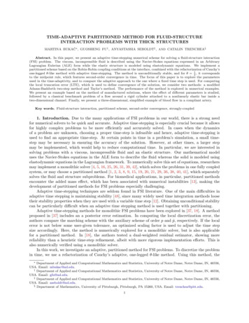
5.1. Example 1. In the first example, we use the method of manufactured solutions to investigatethe performance of Algorithm 1 based on the different parameters in the problem. We define the fluid andstructure domains as ΩF [0, 1] x [0, 0.5] and ΩS [0, 1] x [0.5, 1], respectively. In this example, we assumethat the fluid-structure interaction is linear, that the fluid domain is fixed and that the structure is describedusing a linearly elastic model, given byσS 2µS D(η) λS ( · η)I,(5.1)where µS and λS are Lamé parameters. We define the exact solution as 0.002et x(1 x)y(1 y)η ξ u ,0.001et x(1 x)y(1 y)and p 0.001et (2(1 2x)y(1 y) x(1 x)(1 2y)).The Neumann boundary conditions are imposed at the external boundaries of the structure domain. Atthe left and right boundaries of the fluid domain, we also impose the Neumann conditions while the Dirichlet conditions are imposed at the bottom boundary. The boundary conditions and the forcing terms arecomputed using the exact solution.The coefficients related to the material properties of the fluid and solid, µS , λS , µF , ρS , ρF are all set to1, and parameter θ is set to 21 , in which case we expect the second-order accuracy. To discretize the problemin space, we chose P1 elements for the fluid pressure and P2 elements for the fluid velocity, as well as thedisplacement and velocity of the solid. The final time is set to T 5 s.5.1.1. Choice of Tb. In this section, we investigate the optimal choice of defining the LTE, which isused for time-adaptivity in Algorithm 1. The initial time step is set to τ 0 0.01 s and we use the adaptivitytolerance of δ 10 6 . The adaptivity process begins after two iterations have passed. The tolerance whichcontrols the convergence of the subiterations in Step 1, , is set to ε 10 4 . The combination parameter isdetermined usingα ρS HSHS Eτ 0 ,0τ(1 ν 2 )HF2(5.2)where HS and HF are the height of the solid and fluid domain, respectively, E is the Young’s modulus andν is the Poisson’s ratio. To compute the LTE, we consider both the formula based on the AB2 method (4.1),and the formula based on the Taylor’s method (4.3), as described in Section 4. To determine the size of theLTE, we first setqkTbk kTbη k2 kTbu k2 ,where Tbη is the LTE for the structure displacement, and Tbu is the LTE for the fluid velocity. Figure 5.1 showsthe evolution of the LTEs for the velocity (top-left) and the displacement (bottom-left), the number of trialsover time (top-right), and the evolution of the time step (bottom-right) obtained for this choice of Tb, wherethe LTE is computed using the AB2 method (4.1). We can observe that kTbk is determined by the LTE forthe velocity because of the difference in the magnitudes of Tbη and Tbu . In this case, the simulation endedbefore t 1.5 was reached. The LTE for the fluid velocity exceeded the given tolerance and then starteddecreasing very slowly while the time step was adapting accordingly. Finally, the time step decreased to amachine zero, which caused the simulations to break before the LTE decreased below the given tolerance.As the time step decreased to zero, the LTE for the displacement decreased rapidly as well. The similarbehavior is also obtained when the LTE is computed using the Taylor’s method (4.3), however the figuresare not included for clearer presentation and in order to avoid redundancy.We note that a similar behavior was observed with this definition of kTbk when time-adaptive FSIproblems with thin structures were studied in [11]. Hence, we consider redefining Tb by considering theLTE for the structure displacement only, Tb Tbη . The results obtained with this selection are shown inFigure 5.2. In this case, the simulation is completed successfully using both AB2 and Taylor’s method.8

10 -56number of trials642000.514201.500.510-61.50.3time umber of trialsFig. 5.1: Example 5.1.1: The LTE for the fluid velocity (top-left) and the structure displacement (bottomleft), the total number of trials during the simulation (top-right), andq the evolution of the time step (bottomright). The results are obtained with the LTE defined as kTbk kTbη k2 kTbu k2 and computed using theAB2 method.While the adaptivity is controlled by the LTE for the displacement, we note that the LTE for the velocityremains bounded in both cases since the problem is coupled. Using AB2 method, at most 4 trials are neededto advance in time, with the average of 1.18 trials. When Taylor’s method is used, no more than 2 trials areneeded at any point in time, with the average of 1.4815 trials. The Taylor’s method results in larger valuesof the time step but larger number of average trials compared to the AB2 method. In both cases, the timestep does not approach zero. Based on our results in this section, we use Tb Tbη in the remainder of thepaper.5.1.2. Choice of α. The combination parameter, α, used in the partitioning between the fluid andsolid problems, is often determined heuristically, for example using (5.2). Since there are a variety of waysin which it can be computed, in this section we focus on the effects of the different values of α on theperformance of Algorithm 1. We set τ 0 0.01 as in Example 5.1.1, and use δ 10 6 . As it was shownin [10] that needs to be reduced at the same rate as the time step in order to obtain the optimal rate ofconvergence, we use the following formula to compute : n 1 min{ n τ n 1 /τ n , 0 }.(5.3)starting from 0 10 4 . While the formula is based on (3.2), an outer min{} is added to prevent thetolerance from becoming too large, which could have a significant effect on the accuracy.nTo test the effects of α, we use values of 100, 500, 1000, and αF, which is adapted together with thetime step usingαn HS Eτ nρ S HS .τn(1 ν 2 )HF2(5.4)The LTE is defined as Tb Tbη and computed using formulas based on both AB2 and Taylor’s methods,which are detailed in Section 4.Table 5.1 shows the average number of subiterations required in Step 1 and the average number of trialsused in the time adaptivity. A wide range of the number of subiterations is observed for both AB2 and9

10 -6number of .5time stepAB2Taylor10.5000time10 -62312345timeAB2Taylor0.40.200204060number of trialsFig. 5.2: Example 5.1.1: The LTE for the fluid velocity (top-left) and the structure displacement (bottomleft), the total number of trials during the simulation (top-right), and the evolution of the time step (bottomright). The results are obtained with the LTE defined as Tb Tbη .Taylor’s methods, where in both cases, the smallest value is obtained when α αn . The number of trialsused in the time adaptivity shows very small variability when different values of α are used. In fact, the onlyslight difference in the results is obtained when AB2 method is used with α αn .α 100α 500α 1000α αnAB2# of subiterations24.871445.556.87147.35714# of trials1.16671.16671.16671.007Taylor# of subiterations # of .4815Table 5.1: Example 5.1.2: The average number of subiterations in Step 1 per time step and the averagenumber of trials used for time-adaptivity obtained using the AB2 and Taylor’s methods for the computationof LTE, and different values of the combination parameter, α.Our results indicate that formula (5.4) provides a good choice for the combinati

The remainder of this paper is as follows: Section 2 introduces the problem setting, with the numerical solver detailed out in Section 3. The LTE and its computation is established in Section 4. The numerical examples are presented in Section 5, and the conclusions are drawn in Section 6. 2. Problem setting. Suppose that a bounded, deformable .