WIXLIB

Normalization normalizing the data/random variable is definedZi Xi X̄s– empirical mean 0, empirical standard deviation 1– distribution centered around 0 and data have units # of standard deviations away from theoriginal mean example: Z1 2 means that the data point is 2 standard deviations larger than the originalmean normalization makes non-comparable data comparableEmpirical Covariance & Correlation Let (Xi , Yi ) pairs of data empirical covariance is defined asn1 X1Cov(X, Y ) (Xi X̄)(Yi Ȳ ) n 1 i 1n 1nX!Xi Yi nX̄ Ȳi 1– has units of X units of Y correlation is defined asCor(X, Y ) Cov(X, Y )Sx Sywhere Sx and Sy are the estimates of standard deviations for the X observations and Y observations,respectively––––the value is effectively the covariance standardized into a unit-less quantityCor(X, Y ) Cor(Y, X) 1 Cor(X, Y ) 1Cor(X, Y ) 1 and Cor(X, Y ) 1 only when the X or Y observations fall perfectly on a positiveor negative sloped line, respectively– Cor(X, Y ) measures the strength of the linear relationship between the X and Y data, withstronger relationships as Cor(X, Y ) heads towards -1 or 1– Cor(X, Y ) 0 implies no linear relationship5

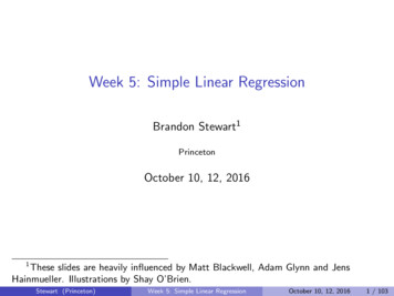
Dalton’s Data and Least Squares collected data from 1885 in UsingR packagepredicting children’s heights from parents’ heightobservations from the marginal/individual parent/children distributionslooking only at the children’s dataset to find the best predictor– “middle” of children’s dataset best predictor– “middle” center of mass mean of the dataset Let Yi height of child i for i 1, . . . , n 928, the “middle” µ such thatnX(Yi µ)2i 1 µ Ȳ for the above sum to be the smallest least squares empirical mean– Note: manipulate function can help to show this# load necessary packages/install if neededlibrary(ggplot2); library(UsingR); data(galton)# function to plot the histogramsmyHist - function(mu){# calculate the mean squaresmse - mean((galton child - mu) 2)# plot histogramg - ggplot(galton, aes(x child)) geom histogram(fill "salmon",colour "black", binwidth 1)# add vertical line marking the center value mug - g geom vline(xintercept mu, size 2)g - g ggtitle(paste("mu ", mu, ", MSE ", round(mse, 2), sep ""))g}# manipulate allows the user to change the variable mu to see how the mean squares changes#library(manipulate); manipulate(myHist(mu), mu slider(62, 74, step 0.5))]# plot the correct graphmyHist(mean(galton child))mu 68.0884698275862, MSE 6.33count150100500606570child in order to visualize the parent-child height relationship, a scatter plot can be used675

Note: because there are multiple data points for the same parent/child combination, a third dimension(size of point) should be used when constructing the scatter plotlibrary(dplyr)# constructs table for different combination of parent-child heightfreqData - as.data.frame(table(galton child, galton parent))names(freqData) - c("child (in)", "parent (in)", "freq")# convert to numeric valuesfreqData child - as.numeric(as.character(freqData child))freqData parent - as.numeric(as.character(freqData parent))# filter to only meaningful combinationsg - ggplot(filter(freqData, freq 0), aes(x parent, y child))g - g scale size(range c(2, 20), guide "none" )# plot grey circles slightly larger than data as base (achieve an outline effect)g - g geom point(colour "grey50", aes(size freq 10, show guide FALSE))# plot the accurate data pointsg - g geom point(aes(colour freq, size freq))# change the color gradient from default to lightblue - whiteg - g scale colour gradient(low "lightblue", high "white")gfreq70child403020106564666870parent772

Derivation for Least Squares Empirical Mean (Finding the Minimum) Let Xi regressor/predictor, and Yi outcome/result so we want to minimize the the squares:nX(Yi µ)2i 1 Proof is as followsnnXX(Yi µ)2 (Yi Ȳ Ȳ µ)2 added Ȳ which is adding 0 to the original equationi 1i 1(expanding the terms) nX(Yi Ȳ )2 2i 1(simplif ying) nXnX(Yi Ȳ )(Ȳ µ) i 1nX(Ȳ µ)2 (Yi Ȳ ), (Ȳ µ) are the termsi 1nnXX(Yi Ȳ )2 2(Ȳ µ)(Yi Ȳ ) (Ȳ µ)2 (Ȳ µ) does not depend on ii 1i 1i 1nnnnXXXXȲ is equivalent to nȲ(Ȳ µ)2 Yi nȲ ) (Yi Ȳ )2 2(Ȳ µ)((simplif ying) i 1i 1i 1i 1nnnnXXXXYi nȲYi nȲ 0 since(Ȳ µ)2 (Yi Ȳ )2 (simplif ying) i 1nX(Yi µ)2 nX(Yi Ȳ )2 i 1i 1i 1nXi 1i 1(Ȳ µ)2 is always 0 so we can take it out to form the inequalityi 1– because of the inequality above, to minimize the sum of the squaresequal to µPni 1 (Yi µ)2 , Ȳ must be An alternative approach to finding the minimum is taking the derivative with respect to µPnd( i 1 (Yi µ)2 ) 0 setting this equal to 0 to find minimumdµnX(Yi µ) 0 divide by -2 on both sides and move µ term over to the right 2i 1nXi 1Yi nXµ for the two sums to be equal, all the terms must be equali 1Yi µ8

Regression through the Origin Let Xi parents’ heights (regressor) and Yi children’s heights (outcome) find a line with slope β that passes through the origin at (0,0)Yi Xi βsuch that it minimizesnX(Yi Xi β)2i 1 Note: it is generally a bad practice forcing the line through (0, 0) Centering Data/Gaussian Elimination– Note: this is different from regression through the origin, because it is effectively moving theregression line– subtracting the means from the Xi s and Yi s moves the origin (reorienting the axes) to the centerof the data set so that a regression line can be constructed– Note: the line constructed here has an equivalent slope as the result from linear regression withintercept9

Derivation for β Let Y βX, and β̂ estimate of β, the slope of the least square regression linenX(Yi Xi β)2 i 1(expanding the terms) n hXi 1nX(Yi Xi β̂) (Xi β̂ Xi β)(Yi Xi β̂)2 2i 1nX(Yi Xi β)2 i 1nXnXi2 added Xi β̂ is effectively adding zero(Yi Xi β̂)(Xi β̂ Xi β) i 1nX(Xi β̂ Xi β)2i 1nnXX(Yi Xi β̂)2 2(Yi Xi β̂)(Xi β̂ Xi β) (Xi β̂ Xi β)2 is always positivei 1i 1i 1(ignoring the second term f or now, f or β̂ to be the minimizer of the squares,nXthe f ollowing must be true)nX(Yi Xi β)2 (Yi Xi β̂)2 every other β value creates a least square criteria that is β̂i 1i 1nX(this means) 2(simplif ying) (simplif ying) (Yi Xi β̂)(Xi β̂ Xi β) 0i 1nX(Yi Xi β̂)Xi (β̂ β) 0 (β̂ β) does not depend on ii 1nX(Yi Xi β̂)Xi 0i 1PnYi Xi(solving f or β̂) β̂ Pi 1n2 βi 1 Xi example– Let X1 , X2 , . . . , Xn 1nnXX(Yi Xi β)2 (Yi β)2i 1i 1PnPnPnYi XiYiYii 1i 1 β̂ Pn Pn i 1 Ȳ2ni 1 Xii 1 1– Note: this is the result from our previous derivation for least squares empirical mean10

Finding the Best Fit Line (Ordinary Least Squares) best fitted line for predictor, X, and outcome, Y is derived from the least squaresnX{Yi (β0 β1 Xi )}2i 1 each of the data point contributes equally to the error between the their locations and the regressionline goal of regression is to minimize this errorLeast Squares Model Fit model fit Y β0 β1 X through the data pairs (Xi , Yi ) where Yi as the outcome– Note: this is the model that we use to guide our estimated best fit (see below) best fit line with estimated slope and intercept (X as predictor, Y as outcome) Y β̂0 β̂1 Xwhereβ̂1 Cor(Y, X)Sd(Y )Sd(X)β̂0 Ȳ β̂1 X̄– [slope] β̂1 has the units of Y /X Cor(Y, X) unit-less Sd(Y ) has units of Y Sd(X) has units of X– [intercept] β̂0 has the units of Y– the line passes through the point (X̄, Ȳ ) this is evident from equation for β0 (rearrange equation) best fit line with X as outcome and Y as predictor has slope, β̂1 Cor(Y, X)Sd(X)/Sd(Y ). slope of best fit line slope of best fit line through the origin for centered data (Xi X̄, Yi Ȳ )Yi Ȳi X̄ slope of best fit line for normalized the data, { XSd(X) , Sd(Y ) } Cor(Y, X)11

Derivation for β0 and β1 Let Y β0 β1 X, and β̂0 /β̂1 estimates β0 /β1 , the intercept and slope of the least square regressionline, respectivelynnXX(Yi β0 β1 Xi )2 (Yi β0 )2i 1solution f orwhere Yi Yi β1 Xii 1nX(Yi Pn2 β0 ) β̂0 i 1Yi ni 1PnPni 1 Yi β1 XinPni 1 Xinn β̂0 Ȳ β1 X̄nnXX 22 (Yi β0 β1 Xi ) Yi (Ȳ β1 X̄) β1 Xi β̂0 i 1i 1Yi β1i 1nX 2 (Yi Ȳ ) (Xi X̄)β1i 1nX 2 Ỹi X̃i β1where Ỹi Yi Ȳ , X̃i Xi X̄i 1PnỸi X̃i(Yi Ȳ )(Xi X̄) β̂1 Pi 12 Pnn2i 1 (Xi X̄)i 1 X̃iCov(Y, X)(Yi Ȳ )(Xi X̄)/(n 1) β̂1 Pn2 /(n 1)V ar(X)(X X̄)ii 1Sd(Y ) β̂1 Cor(Y, X)Sd(X) β̂0 Ȳ β̂1 X̄Examples and R Commands β̂0 and β̂1 can be manually calculated through the above formulas coef(lm(y x))) R command to run the least square regression model on the data with y as theoutcome, and x as the regressor– coef() returns the slope and intercept coefficients of the lm results# outcomey - galton child# regressorx - galton parent# slopebeta1 - cor(y, x) * sd(y) / sd(x)# interceptbeta0 - mean(y) - beta1 * mean(x)# results are the same as using the lm commandresults - rbind("manual" c(beta0, beta1), "lm(y x)" coef(lm(y x)))# set column namescolnames(results) - c("intercept", "slope")# print resultsresults12

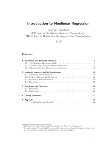
##interceptslope## manual23.94153 0.6462906## lm(y x) 23.94153 0.6462906 slope of the best fit line slope of best fit line through the origin for centered data lm(y x - 1) forces a regression line to go through the origin (0, 0)# centering yyc - y - mean(y)# centering xxc - x - mean(x)# slopebeta1 - sum(yc * xc) / sum(xc 2)# results are the same as using the lm commandresults - rbind("centered data (manual)" beta1, "lm(y x)" coef(lm(y x))[2],"lm(yc xc - 1)" coef(lm(yc xc - 1))[1])# set column namescolnames(results) - c("slope")# print resultsresults##slope## centered data (manual) 0.6462906## lm(y x)0.6462906## lm(yc xc - 1)0.6462906 slope of best fit line for normalized the data Cor(Y, X)# normalize yyn - (y - mean(y))/sd(y)# normalize xxn - (x - mean(x))/sd(x)# compare correlationsresults - rbind("cor(y, x)" cor(y, x), "cor(yn, xn)" cor(yn, xn),"slope" coef(lm(yn xn))[2])# print resultsresults##xn## cor(y, x)0.4587624## cor(yn, xn) 0.4587624## slope0.4587624 geom smooth(method "lm", formula y x) function in ggplot2 adds regression line and confidence interval to graph– formula y x default for the line (argument can be eliminated if y x produces the line youwant)# constructs table for different combination of parent-child heightfreqData - as.data.frame(table(galton child, galton parent))names(freqData) - c("child (in)", "parent (in)", "freq")13

# convert to numeric valuesfreqData child - as.numeric(as.character(freqData child))freqData parent - as.numeric(as.character(freqData parent))g - ggplot(filter(freqData, freq 0), aes(x parent, y child))g - g scale size(range c(2, 20), guide "none" )g - g geom point(colour "grey50", aes(size freq 10, show guide FALSE))g - g geom point(aes(colour freq, size freq))g - g scale colour gradient(low "lightblue", high "white")g - g geom smooth(method "lm", formula y x)gfreq70child403020106564666870parent1472

Regression to the Mean first investigated by Francis Galton in the paper “Regression towards mediocrity in hereditary stature”The Journal of the Anthropological Institute of Great Britain and Ireland , Vol. 15, (1886) regression to the mean was invented by Fancis Galton to capture the following phenomena––––children of tall parents tend to be tall, but not as tall as their parentschildren of short parents tend to be short, but not as short as their parentsparents of very short children, tend to be short, but not as short as their childparents of very tall children, tend to be tall, but not as tall as their children in thinking of the extremes, the following are true– P (Y x X x) gets bigger as x heads to very large values in other words, given that the value of X is already very large (extreme), the chance that thevalue of Y is as large or larger than that of X is small (unlikely)– similarly, P (Y x X x) gets bigger as x heads to very small values in other words, given that the value of X is already very small (extreme), the chance that thevalue of Y is as small or smaller than that of X is small (unlikely) when constructing regression lines between X and Y , the line represents the intrinsic relationship(“mean”) between the variables, but does not capture the extremes (“noise”)– unless Cor(Y, X) 1, the regression line or the intrinsic part of the relationship between variableswon’t capture all of the variation (some noise exists)Dalton’s Investigation on Regression to the Mean both X, child’s heights, and Y , parent’s heights, are normalized so that they mean of 0 and varianceof 1 regression lines must pass (X̄, Ȳ ) or (0, 0) in this case slope of regression line Cor(Y, X) regardless of which variable is the outcome/regressor (becausestandard deviations of both variables 1)– Note: however, for both regression lines to be plotted on the same graph, the second line’s slopemust be 1/Cor(Y, X) because the two relationships have flipped axes# load father.son datadata(father.son)# normalize son's heighty - (father.son sheight - mean(father.son sheight)) / sd(father.son sheight)# normalize father's heightx - (father.son fheight - mean(father.son fheight)) / sd(father.son fheight)# calculate correlationrho - cor(x, y)# plot the relationship between the twog ggplot(data.frame(x x, y y), aes(x x, y y))g g geom point(size 3, alpha .2, colour "black")g g geom point(size 2, alpha .2, colour "red")g g xlim(-4, 4) ylim(-4, 4)# reference line for perfect correlation between# variables (data points will like on diagonal line)g g geom abline(position "identity")# if there is no correlation between the two variables,# the data points will lie on horizontal/vertical lines15

1x4,x)y(ry g g geom vline(xintercept 0) g geom hline(yintercept 0)plot the actual correlation for both g geom abline(intercept 0, slope rho, size 2) g geom abline(intercept 0, slope 1 / rho, size 2)add appropriate labels g xlab("Father's height, normalized") g ylab("Son's height, normalized") g geom text(x 3.8, y 1.6, label "x y", angle 25) geom text(x 3.2, y 3.6, label "cor(y,x) 1", angle 35) geom text(x 1.6, y 3.8, label "y x", angle 60)coSon's height, normalizedgg#gg#ggg2x y0 2 4 4 202Father's height, normalized164

Statistical Linear Regression Models goal is use statistics to draw inferences generalize from data to population through models probabilistic model for linear regressionYi β0 β1 Xi iwhere i represents the sampling errors and is assumed to be iid N (0, σ 2 ) this model has the following properties– E[Yi Xi xi ] E[β0 ] E[β1 xi ] E[ i ] µi β0 β1 xi– V ar(Yi Xi xi ) V ar(β0 β1 xi ) V ar( i ) V ar( i ) σ 2 β0 β1 xi line constant/no variance it can then be said to have Yi as independent N (µ, σ 2 ), where µ β0 β1 xi – likelihood equivalentmodel– likelihood given the outcome, what is the probability? in this case, the likelihood is as followsL(β0 , β1 , σ) n Y2 1/2(2πσ )i 1 1exp 2 (yi µi )22σ where µi β0 β1 xi above is the probability density function of n samples from the normal distribution this is because the regression line is normally distributed due to i– maximum likelihood estimator (MLE) most likely estimate of the population parameter/probability in this case, the maximum likelihood -2 minimum natural log (ln, base e) likelihood 2 log L(β0 , β1 , σ) n log(2πσ 2 ) n1 X(yi µi )2σ 2 i 1· since everything else is constant, minimizing this function would only depend onµi )2 , which from our previous derivations yields µ̂i β0 β1 x̂iPni 1 (yi maximum likelihood estimate µi β0 β1 xiInterpreting Regression Coefficients for the linear regression lineYi β0 β1 Xi iMLE for β0 and β1 are as followsβ̂1 Cor(Y, X)Sd(Y )Sd(X)β̂0 Ȳ β̂1 X̄ β0 expected value of the outcome/response when the predictor is 0E[Y X 0] β0 β1 0 β0– Note: X 0 may not always be of interest as it may be impossible/outside of data range (i.eblood pressure, height etc.)17

– it may be useful to move the intercept at timesYi β0 β1 Xi i β0 aβ1 β1 (Xi a) i β̃0 β1 (Xi a) iwhereβ̃0 β0 aβ1– Note: shifting X values by value a changes the intercept, but not the slope– often, a is set to X̄ so that the intercept is interpreted as the expected response at the average Xvalue β1 expected change in outcome/response for a 1 unit change in the predictorE[Y X x 1] E[Y X x] β0 β1 (x 1) (β0 β1 x) β1– sometimes it is useful to change the units of XYi β0 β1 Xi iβ1 β0 (Xi a) ia β0 β̃1 (Xi a) i– multiplication of X by a factor a results in dividing the coefficient by a factor of a– example: X height in mY weight in kgβ1 has units of kg/mconverting X to cm multiplying X by 100 cmmthis mean β1 has to be divided by 100 cmm for the correct units.X m 1001 mkgcm (100 X)cm and β1 mm100 cm β1100 kgcm 95% confidence intervals for the coefficients can be constructed from the coefficients themselves andtheir standard errors (from summary(lm))– use the resulting intervals to evaluate the significance of the resultsUse Regression Coefficients for Prediction for observed values of the predictor, X1 , X2 , . . . , Xn , the prediction of the outcome/response is as followsµ̂i Ŷi β̂0 β̂1 Xwhere µi describes a point on the regression lineExample and R Commands diamond dataset from UsingR package– diamond prices in Singapore Dollars, diamond weight in carats (standard measure of diamondmass, 0.2g) lm(price I(carat - mean(carat)), data diamond) mean centered linear regression– Note: arithmetic operations must be enclosed in I() to work18

predict(fitModel, newdata data.frame(carat c(0, 1, 2))) returns predicted outcome fromthe given model (linear in our case) at the provided points within the newdata data frame– if newdata is unspecified (argument omitted), then predict function will return predicted valuesfor all values of the predictor (x variable, carat in this case) Note: newdata has to be a dataframe, and the values you would like to predict (x variable,carat in this case) has to be specified, or the system won’t know what to do wit

Regression Models Course Notes Xing Su Contents IntroductiontoRegression. . . . . . . . . . . . . . . . . . . . . . . . . . . . . . . . . . . . . . . . .4