Transcription
Model Predictive ControlToolboxFor Use with MATLAB Alberto BemporadManfred MorariN. Lawrence RickerUser’s GuideVersion 2
How to Contact The Newsgroupinfo@mathworks.comTechnical supportProduct enhancement suggestionsBug reportsDocumentation error reportsOrder status, license renewals, passcodesSales, pricing, and general information508-647-7000Phone508-647-7001FaxThe MathWorks, Inc.3 Apple Hill DriveNatick, MA athworks.comFor contact information about worldwide offices, see the MathWorks Web site.Model Predictive Control Toolbox User’s Guide COPYRIGHT 1995-2005 by The MathWorks, Inc.The software described in this document is furnished under a license agreement. The software may be usedor copied only under the terms of the license agreement. No part of this manual may be photocopied or reproduced in any form without prior written consent from The MathWorks, Inc.FEDERAL ACQUISITION: This provision applies to all acquisitions of the Program and Documentation by,for, or through the federal government of the United States. By accepting delivery of the Program orDocumentation, the government hereby agrees that this software or documentation qualifies as commercialcomputer software or commercial computer software documentation as such terms are used or defined inFAR 12.212, DFARS Part 227.72, and DFARS 252.227-7014. Accordingly, the terms and conditions of thisAgreement and only those rights specified in this Agreement, shall pertain to and govern the use,modification, reproduction, release, performance, display, and disclosure of the Program and Documentationby the federal government (or other entity acquiring for or through the federal government) and shallsupersede any conflicting contractual terms or conditions. If this License fails to meet the government'sneeds or is inconsistent in any respect with federal procurement law, the government agrees to return theProgram and Documentation, unused, to The MathWorks, Inc.MATLAB, Simulink, Stateflow, Handle Graphics, Real-Time Workshop, and xPC TargetBox are registeredtrademarks of The MathWorks, Inc.Other product or brand names are trademarks or registered trademarks of their respectiveholders.Printing History: January 1995First printingOctober 1998Online onlyJune 2004Online onlyRevised for Version 2.0 (Release 14)October 2004Online onlyRevised for Version 2.1 (Release 14SP1)March 2005Online onlyRevised for Version 2.2 (Release 14SP2)
ContentsIntroduction1What Is the Model Predictive Control Toolbox? . . . . . . . . . . 1-2Model Predictive Control of a SISO Plant . . . . . . . . . . . . . . . 1-3A Typical Sampling Instant . . . . . . . . . . . . . . . . . . . . . . . . . . . . 1-5Prediction and Control Horizons . . . . . . . . . . . . . . . . . . . . . . . . 1-8MIMO Plants . . . . . . . . . . . . . . . . . . . . . . . . . . . . . . . . . . . . . . . .Optimization and Constraints . . . . . . . . . . . . . . . . . . . . . . . . .State Estimation . . . . . . . . . . . . . . . . . . . . . . . . . . . . . . . . . . . .Blocking . . . . . . . . . . . . . . . . . . . . . . . . . . . . . . . . . . . . . . . . . . .1-101-101-131-14MPC Problem Setup2Prediction Model . . . . . . . . . . . . . . . . . . . . . . . . . . . . . . . . . . . . . 2-2Offsets . . . . . . . . . . . . . . . . . . . . . . . . . . . . . . . . . . . . . . . . . . . . . 2-4Optimization Problem . . . . . . . . . . . . . . . . . . . . . . . . . . . . . . . . . 2-5State Estimation . . . . . . . . . . . . . . . . . . . . . . . . . . . . . . . . . . . . . .Measurement Noise Model . . . . . . . . . . . . . . . . . . . . . . . . . . . . .Output Disturbance Model . . . . . . . . . . . . . . . . . . . . . . . . . . . . .State Observer . . . . . . . . . . . . . . . . . . . . . . . . . . . . . . . . . . . . . . .2-82-82-92-9QP Matrices . . . . . . . . . . . . . . . . . . . . . . . . . . . . . . . . . . . . . . . . .Prediction . . . . . . . . . . . . . . . . . . . . . . . . . . . . . . . . . . . . . . . . . .Optimization Variables . . . . . . . . . . . . . . . . . . . . . . . . . . . . . . .Cost Function . . . . . . . . . . . . . . . . . . . . . . . . . . . . . . . . . . . . . . .Constraints . . . . . . . . . . . . . . . . . . . . . . . . . . . . . . . . . . . . . . . .2-122-122-132-152-16MPC Computation . . . . . . . . . . . . . . . . . . . . . . . . . . . . . . . . . . . 2-18i
Unconstrained MPC . . . . . . . . . . . . . . . . . . . . . . . . . . . . . . . . . . 2-18Constrained MPC . . . . . . . . . . . . . . . . . . . . . . . . . . . . . . . . . . . . 2-18Using Identified Models . . . . . . . . . . . . . . . . . . . . . . . . . . . . . . 2-19MPC Simulink Library3MPC Controller Block . . . . . . . . . . . . . . . . . . . . . . . . . . . . . . . . .Opening the Library . . . . . . . . . . . . . . . . . . . . . . . . . . . . . . . . . .MPC Controller Block Mask . . . . . . . . . . . . . . . . . . . . . . . . . . . .Look Ahead and Signals from the Workspace . . . . . . . . . . . . . .Initialization . . . . . . . . . . . . . . . . . . . . . . . . . . . . . . . . . . . . . . . . .Using the MPC Toolbox with Real-Time Workshop . . . . . . . .3-23-23-33-43-53-5Case-Study Examples4Servomechanism Controller . . . . . . . . . . . . . . . . . . . . . . . . . . . 4-2System Model . . . . . . . . . . . . . . . . . . . . . . . . . . . . . . . . . . . . . . . . 4-2Control Objectives and Constraints . . . . . . . . . . . . . . . . . . . . . . 4-4Defining the Plant Model . . . . . . . . . . . . . . . . . . . . . . . . . . . . . . 4-4Controller Design Using MPCTOOL . . . . . . . . . . . . . . . . . . . . . 4-5Using MPC Toolbox Commands . . . . . . . . . . . . . . . . . . . . . . . . 4-22Using MPC Tools in Simulink . . . . . . . . . . . . . . . . . . . . . . . . . . 4-26Paper Machine Process Control . . . . . . . . . . . . . . . . . . . . . . .Linearizing the Nonlinear Model . . . . . . . . . . . . . . . . . . . . . . .MPC Design . . . . . . . . . . . . . . . . . . . . . . . . . . . . . . . . . . . . . . . .Controlling the Nonlinear Plant in Simulink . . . . . . . . . . . . . .4-304-314-334-39Reference . . . . . . . . . . . . . . . . . . . . . . . . . . . . . . . . . . . . . . . . . . . 4-43iiContents
The Design Tool5Opening the MPC Design Tool . . . . . . . . . . . . . . . . . . . . . . . . . . 5-2The Menu Bar . . . . . . . . . . . . . . . . . . . . . . . . . . . . . . . . . . . . . . . . 5-3File Menu . . . . . . . . . . . . . . . . . . . . . . . . . . . . . . . . . . . . . . . . . . . 5-3MPC Menu . . . . . . . . . . . . . . . . . . . . . . . . . . . . . . . . . . . . . . . . . . 5-4The Tool Bar . . . . . . . . . . . . . . . . . . . . . . . . . . . . . . . . . . . . . . . . . . 5-6The Tree View . . . . . . . . . . . . . . . . . . . . . . . . . . . . . . . . . . . . . . . . 5-7Node Types . . . . . . . . . . . . . . . . . . . . . . . . . . . . . . . . . . . . . . . . . . 5-7Renaming a Node . . . . . . . . . . . . . . . . . . . . . . . . . . . . . . . . . . . . . 5-8Importing a Plant Model . . . . . . . . . . . . . . . . . . . . . . . . . . . . . . . 5-9Import from . . . . . . . . . . . . . . . . . . . . . . . . . . . . . . . . . . . . . . . . 5-10Import to . . . . . . . . . . . . . . . . . . . . . . . . . . . . . . . . . . . . . . . . . . . 5-11Buttons . . . . . . . . . . . . . . . . . . . . . . . . . . . . . . . . . . . . . . . . . . . . 5-11Importing a Linearized Plant Model . . . . . . . . . . . . . . . . . . . . . 5-12Importing a Controller . . . . . . . . . . . . . . . . . . . . . . . . . . . . . . .Import from . . . . . . . . . . . . . . . . . . . . . . . . . . . . . . . . . . . . . . . .Import to . . . . . . . . . . . . . . . . . . . . . . . . . . . . . . . . . . . . . . . . . . .Buttons . . . . . . . . . . . . . . . . . . . . . . . . . . . . . . . . . . . . . . . . . . . .5-155-165-175-17Exporting a Controller . . . . . . . . . . . . . . . . . . . . . . . . . . . . . . . 5-19Dialog Options . . . . . . . . . . . . . . . . . . . . . . . . . . . . . . . . . . . . . . 5-19Buttons . . . . . . . . . . . . . . . . . . . . . . . . . . . . . . . . . . . . . . . . . . . . 5-20Signal Definition View . . . . . . . . . . . . . . . . . . . . . . . . . . . . . . . .MPC Structure Overview . . . . . . . . . . . . . . . . . . . . . . . . . . . . .Buttons . . . . . . . . . . . . . . . . . . . . . . . . . . . . . . . . . . . . . . . . . . . .Signal Properties Tables . . . . . . . . . . . . . . . . . . . . . . . . . . . . . .Right-Click Menu Options . . . . . . . . . . . . . . . . . . . . . . . . . . . . .5-215-225-225-225-25Plant Models View . . . . . . . . . . . . . . . . . . . . . . . . . . . . . . . . . . .Plant Models List . . . . . . . . . . . . . . . . . . . . . . . . . . . . . . . . . . . .Model Details . . . . . . . . . . . . . . . . . . . . . . . . . . . . . . . . . . . . . . .Additional Notes . . . . . . . . . . . . . . . . . . . . . . . . . . . . . . . . . . . .5-265-275-275-28iii
Buttons . . . . . . . . . . . . . . . . . . . . . . . . . . . . . . . . . . . . . . . . . . . . 5-28Right-Click Options . . . . . . . . . . . . . . . . . . . . . . . . . . . . . . . . . . 5-28ivContentsControllers View . . . . . . . . . . . . . . . . . . . . . . . . . . . . . . . . . . . . .Controllers List . . . . . . . . . . . . . . . . . . . . . . . . . . . . . . . . . . . . .Controller Details . . . . . . . . . . . . . . . . . . . . . . . . . . . . . . . . . . . .Additional Notes . . . . . . . . . . . . . . . . . . . . . . . . . . . . . . . . . . . .Buttons . . . . . . . . . . . . . . . . . . . . . . . . . . . . . . . . . . . . . . . . . . . .Right-Click Options . . . . . . . . . . . . . . . . . . . . . . . . . . . . . . . . . .5-295-305-315-315-315-32Simulation Scenarios List . . . . . . . . . . . . . . . . . . . . . . . . . . . . .Scenarios List . . . . . . . . . . . . . . . . . . . . . . . . . . . . . . . . . . . . . . .Scenario Details . . . . . . . . . . . . . . . . . . . . . . . . . . . . . . . . . . . . .Additional Notes . . . . . . . . . . . . . . . . . . . . . . . . . . . . . . . . . . . .Buttons . . . . . . . . . . . . . . . . . . . . . . . . . . . . . . . . . . . . . . . . . . . .Right-Click Options . . . . . . . . . . . . . . . . . . . . . . . . . . . . . . . . . .5-335-345-355-355-355-35Controller Specifications View . . . . . . . . . . . . . . . . . . . . . . . .Model and Horizons Tab . . . . . . . . . . . . . . . . . . . . . . . . . . . . . .Constraints Tab . . . . . . . . . . . . . . . . . . . . . . . . . . . . . . . . . . . . .Constraint Softening . . . . . . . . . . . . . . . . . . . . . . . . . . . . . . . . .Weight Tuning Tab . . . . . . . . . . . . . . . . . . . . . . . . . . . . . . . . . .Estimation Tab . . . . . . . . . . . . . . . . . . . . . . . . . . . . . . . . . . . . . .Right-Click Menus . . . . . . . . . . . . . . . . . . . . . . . . . . . . . . . . . . .5-365-365-405-435-475-505-58Simulation Scenario View . . . . . . . . . . . . . . . . . . . . . . . . . . . .Simulation Settings . . . . . . . . . . . . . . . . . . . . . . . . . . . . . . . . . .Setpoints . . . . . . . . . . . . . . . . . . . . . . . . . . . . . . . . . . . . . . . . . . .Measured Disturbances . . . . . . . . . . . . . . . . . . . . . . . . . . . . . . .Unmeasured Disturbances . . . . . . . . . . . . . . . . . . . . . . . . . . . .Signal Type Settings . . . . . . . . . . . . . . . . . . . . . . . . . . . . . . . . .Simulation Button . . . . . . . . . . . . . . . . . . . . . . . . . . . . . . . . . . .Right-Click Menus . . . . . . . . . . . . . . . . . . . . . . . . . . . . . . . . . . .5-595-605-605-615-625-645-655-65Response Plots . . . . . . . . . . . . . . . . . . . . . . . . . . . . . . . . . . . . . . .Data Markers . . . . . . . . . . . . . . . . . . . . . . . . . . . . . . . . . . . . . . .Displaying Multiple Scenarios . . . . . . . . . . . . . . . . . . . . . . . . .Viewing Selected Variables . . . . . . . . . . . . . . . . . . . . . . . . . . . .Grouping Variables in a Single Plot . . . . . . . . . . . . . . . . . . . . .5-675-675-695-705-70
Normalizing Response Amplitudes . . . . . . . . . . . . . . . . . . . . . . 5-71Function Reference6Functions — Categorical List . . . . . . . . . . . . . . . . . . . . . . . . . .MPC Controller . . . . . . . . . . . . . . . . . . . . . . . . . . . . . . . . . . . . . .MPC Controller Characteristics . . . . . . . . . . . . . . . . . . . . . . . . .Linear Behavior of MPC Controller . . . . . . . . . . . . . . . . . . . . . .MPC State . . . . . . . . . . . . . . . . . . . . . . . . . . . . . . . . . . . . . . . . . .MPC Computation and Simulation . . . . . . . . . . . . . . . . . . . . . . .State Estimation . . . . . . . . . . . . . . . . . . . . . . . . . . . . . . . . . . . . .Quadratic Programming . . . . . . . . . . . . . . . . . . . . . . . . . . . . . . .6-26-26-26-36-36-36-46-4Functions — Alphabetical List . . . . . . . . . . . . . . . . . . . . . . . . . 6-5Block Reference7Blocks — Alphabetical List . . . . . . . . . . . . . . . . . . . . . . . . . . . . . 7-2Object Reference8MPC Controller Object . . . . . . . . . . . . . . . . . . . . . . . . . . . . . . . . 8-2Construction and Initialization . . . . . . . . . . . . . . . . . . . . . . . . . 8-12MPC State Object . . . . . . . . . . . . . . . . . . . . . . . . . . . . . . . . . . . . 8-13MPC Simulation Options Object . . . . . . . . . . . . . . . . . . . . . . . 8-14v
IndexviContents
1IntroductionWhat Is the Model Predictive Control Toolbox? (p. 1-2) Toolbox overviewModel Predictive Control of a SISO Plant (p. 1-3)Toolbox concepts: horizons, constraints,tuning weightsMIMO Plants (p. 1-10)Extension to plants with multiple inputsand outputs
1IntroductionWhat Is the Model Predictive Control Toolbox?The Model Predictive Control (MPC) Toolbox is a collection of software thathelps you design, analyze, and implement an advanced industrial automationalgorithm. Like other MATLAB tools, it provides a convenient graphical userinterface (GUI) as well as a flexible command syntax that supportscustomization.As its name suggests, MPC automates a target system (the “plant”) bycombining a prediction and a control strategy. An approximate, linear plantmodel provides the prediction. The control strategy compares predicted plantstates to a set of objectives, then adjusts available actuators to achieve theobjectives while respecting the plant’s constraints. Such constraints caninclude the actuators’ physical limits, boundaries of safe operation, and lowerlimits for product quality.MPC’s constraint-tolerance differentiates it from other “optimal control”strategies (e.g., the Linear-Quadratic-Gaussian approach supported in theControl Systems Toolbox). The impetus for this is industrial experiencesuggesting that the drive for profitability often pushes the plant to one or moreconstraints. MPC’s explicit consideration of such factors allows it to allocatethe available plant resources intelligently as the system evolves over time.The MPC Toolbox uses the same powerful linear dynamic modeling tools foundin the Control Systems and System Identification Toolboxes. You can employtransfer functions, state-space matrices, or a combination of the two. You canalso include delays, which are a common feature of industrial plants.If you don’t have a model but can perform experiments, you can use the SystemIdentification Toolbox to develop a data-based model, then exploit it in theMPC Toolbox.If you’d rather use Simulink graphical tools to model your plant, the MPCToolbox provides a Simulink block for that environment. For example, you caneasily linearize a nonlinear Simulink plant, use the linearized model to buildan MPC Controller block, and evaluate its control of the nonlinear plant.Finally,you can use MPC tools in Simulink to develop and test a controlstrategy, then implement it in a real plant using the Real Time Workshop.1-2
Model Predictive Control of a SISO PlantModel Predictive Control of a SISO PlantThe usual MPC Toolbox application involves a plant having multiple inputsand multiple outputs (a MIMO plant).Consider instead the simpler application shown in Figure 1-1 (see summary ofnomenclature in Table 1-1). This plant could be a manufacturing process, suchas a unit operation in an oil refinery, or a device, such as an electric motor. Themain objective is to hold a single output, y , at a reference value (or setpoint), r,by adjusting a single manipulated variable (or actuator) u. This is what isgenerally termed a SISO (single-input single-output) plant. The block labeledMPC represents an MPC Toolbox feedback controller designed to achieve thecontrol objective.The SISO plant actually has multiple inputs, as shown in Figure 1-1. Inaddition to the manipulated variable input, u, there may be a measureddisturbance, v, and an unmeasured disturbance, d.Measured DisturbanceNoiseSetpointryzvvMPCActuatorudPlant yPlantOutput yUnmeasuredDisturbanceMeasured Output (Controlled Variable)Figure 1-1: Block Diagram of a SISO MPC Toolbox ApplicationThe unmeasured disturbance is always present. As shown in Figure 1-1, it isan independent input – not affected by the controller or the plant. It representsall the unknown, unpredictable events that upset plant operation. (In thecontext of Model Predictive Control, it can also represent unmodeleddynamics.) When such an event occurs, the only indication is its effect on themeasured output, y, which is fed back to the controller as shown in Figure 1-1.1-3
1IntroductionTable 1-1: Description of MPC Toolbox SignalsSymbolDescriptiondUnmeasured disturbance. Unknown but for its effecton the plant output. The controller provides feedbackcompensation for such disturbances.rSetpoint (or reference). The target value for the output.uManipulated variable(or actuator). The signal thecontroller adjusts in order to achieve its objectives.vMeasured disturbance (optional). The controllerprovides feedforward compensation for suchdisturbances as they occur to minimize their impact onthe output.yOutput (or controlled variable). The signal to be heldat the setpoint. This is the “true” value, uncorruptedby measurement noise.yMeasured output. Used to estimate the true value, y .zMeasurement noise. Represents electrical noise,sampling errors, drifting calibration, and other effectsthat impair measurement precision and accuracy.Some applications have unmeasured disturbances only. A measureddisturbance, v, is another independent input affecting y . In contrast to d, thecontroller receives the measured v directly, as shown in Figure 1-1 This allowsthe controller to compensate for v’s impact on y immediately rather thanwaiting until the effect appears in the y measurement. This is calledfeedforward control.In other words, an MPC Toolbox design always provides feeback compensationfor unmeasured disturbances and feedforward compensation for any measureddisturbance.1-4
Model Predictive Control of a SISO PlantThe MPC Toolbox design requires a model of the impact that v and u have ony (symbolically, v y and u y ). It uses this plant model to calculate the uadjustments needed to keep y at its setpoint.This calculation considers the effect of any known constraints on theadjustments (typically an actuator upper or lower bound, or a constraint onhow rapidly u can vary). One may also specify bounds on y . These constraintspecifications are a distinguishing feature of an MPC Toolbox design and canbe particularly valuable when one has multiple control objectives to beachieved via multiple adjustments (a MIMO plant). In the context of a SISOsystem, such contraint handling is often termed an anti-windup feature.If the plant model is accurate, the plant responds quickly to adjustments in u,and no constraints are encountered, feedforward compensation can counteractthe impact of v perfectly. In reality, model imperfections, physical limitations,and unmeasured disturbances cause the y to deviate from its setpoint.Therefore, the MPC Toolbox design includes a disturbance model ( d y ) toestimate d and predict its impact on y . It then uses its u y model to calculateappropriate adjustments (feedback). This calculation also considers the knownconstraints.Various noise effects can corrupt the measurement. The signal z in Figure 1-1represents such effects. They could vary randomly with a zero mean, or couldexhibit a non-zero, drifting bias. The MPC Toolbox design uses a z y modelin combination with its d y model to remove the estimated noise component(filtering).The above feedforward/feedback actions comprise the controller’s regulatormode. The MPC Toolbox design also provides a servo mode, i.e., it adjusts usuch that y tracks a time-varying setpoint.The tracking accuracy depends on the plant characteristics (includingconstraints), the accuracy of the u y model, and whether or not futuresetpoint variations can be anticipated, i.e., known in advance. If so, it providesfeedforward compensation for these.A Typical Sampling InstantAn MPC Toolbox design generates a discrete-time controller – one that takesaction at regularly-spaced, discrete time instants. The sampling instants arethe times at which the controller acts. The interval separating successivesampling instants is the sampling period, t (also called the control interval).1-5
1IntroductionThis section provides more details on the events occuring at each EstimatedyminPrediction Horizon, Pumax(b)ControlHorizonPast MovesPlanned Movesumin-4-3-2-1k 1 2 3 4 5 6 7 8 9Sampling InstantsFigure 1-2: Controller State at the kth Sampling InstantFigure 1-2 shows the state of a hypothetical SISO MPC system that has beenoperating for many sampling instants. Integer k represents the currentinstant. The latest measured output, yk, and previous measurements, yk-1, yk-2,., are known and are the filled circles in Figure 1-2(a). If there is a measureddisturbance, its current and past values would be known (not shown).1-6
Model Predictive Control of a SISO PlantFigure 1-2 (b) shows the controller’s previous moves, uk-41, ., uk-1, as filledcircles. As is usually the case, a zero-order hold receives each move from thecontroller and holds it until the next sampling instant, causing the step-wisevariations shown in Figure 1-2 (b).To calculate its next move, uk the controller operates in two phases:1 Estimation. In order to make an intelligent move, the controller needs toknow the current state. This includes the true value of the controlledvariable, y k , and any internal variables that influence the future trend,y k 1 , ., y k P . To accomplish this, the controller uses all past and currentmeasurements and the models u y , d y , w y , and z y . Fordetails, see “Prediction” and “State Estimation”.2 Optimization. Values of setpoints, measured disturbances, and constraintsare specified over a finite horizon of future sampling instants, k 1, k 2, .,k P, where P (a finite integer 1) is the prediction horizon – see Figure 1-2(a). The controller computes M moves uk, uk 1, . uk M-1, where M ( 1, P)is the control horizon – see Figure 1-2 (b). In the hypothetical exampleshown in the figure, P 9 and M 4. The moves are the solution of aconstrained optimization problem. For details of the formulation, seeChapter 2, “Optimization Problem”.In the example, the optimal moves are the four open circles in Figure 1-2 (b),and the controller predicts that the resulting output values will be the nineopen circles in Figure 1-2 (a). Notice that both are within their constraints,u min u k j u max and y min y k i y max .When it’s finished calculating, the controller sends move uk to the plant. Theplant operates with this constant input until the next sampling instant, t timeunits later. The controller then obtains new measurements and totally revisesits plan. This cycle repeats indefinitely.Reformulation at each sampling instant is essential for good control. Thepredictions made during the optimization stage are imperfect. Periodicmeasurement feedback allows the controller to correct for this error and forunexpected disturbances.1-7
1IntroductionPrediction and Control HorizonsYou might wonder why the controller bothers to optimize over P futuresampling periods and calculate M future moves when it discards all but thefirst move in each cycle. Indeed, under certain conditions a controller using P M 1 would be identical to one using P M . More often, however, thehorizon values have an important impact. Some examples follow: Constraints. Given sufficiently long horizons, the controller can “see” apotential constraint and avoid it – or at least minimize its adverse effects.For example, consider the situation depicted below in which one controllerobjective is to keep plant output y below an upper bound ymax. The currentsampling instant is k, and the model predicts the upward trend yk i. If thecontroller were looking P1 steps ahead, it wouldn’t be concerned by theconstraint until more time had elapsed. If the prediction horizon were P2, itwould begin to take corrective action immediately.ymaxyk ikk P1k P2 Plant delays. Suppose that the plant includes a pure time delay equivalentto D sampling instants. In other words, the controller’s current move, uk, hasno effect until yk D 1. In this situation it is essential that P D and M P D, as this forces the controller to consider the full effect of each move.For example, suppose D 5, P 7, M 3, the current time instant is k, andthe three moves to be calculated are uk, uk 1, and uk 2. Moves uk, uk 1 wouldhave some impact within the prediction horizon, but move uk 2 would havenone until yk 8, which is outside. Thus, uk 2 is indeterminant. Setting P 8(or M 2) would allow a unique value to be determined. It would be better toincrease P even more. Other nonminimum phase plants. Consider a SISO plant with aninverse-response, i.e., a plant with a short-term response in one direction,1-8
Model Predictive Control of a SISO Plantbut a longer term response in the opposite direction. The optimization shouldfocus primarily on the longer-term behavior. Otherwise, the controller wouldmove in the wrong direction.Most designers choose P and M such that controller performance is insensitiveto small adjustments in these horizons. Here are typical rules of thumb for alag-dominant, stable process:1 Choose the control interval such that the plant’s open-loop settling time isapproximately 20-30 sampling periods (i.e., the sampling period isapproximately one fifth of the dominant time constant).2 Choose prediction horizon P to be the number of sampling periods used instep 1.3 Use a relatively small control horizon M, e.g., 3-5.If performance is poor, you should examine other aspects of the optimizationproblem and/or check for inaccurate controller predictions.1-9
1IntroductionMIMO PlantsOne advantage of an MPC Toolbox design (relative to classical multi-loopcontrol) is that it generalizes directly to plants having multiple inputs andoutputs. Moreover, the plant can be non-square, i.e., having an unequalnumber of actuators and outputs. Industrial applications involving hundredsof actuators and controller outputs have been reported.The main challenge is to tune the controller to achieve multiple objectives. Forexample, if there are several outputs to be controlled, it might be necessary toprioritize so that the controller provides accurate setpoint tracking for the mostimportant output, sacrificing others when necessary, e.g., when it encountersconstraints. The MPC Toolbox features support such prioritization.Optimization and ConstraintsAs discussed in more detail in Chapter 2, “Optimization Problem”, the MPCToolbox controller solves anoptimization problem much like the LQG optimalcontrol described in the Control System Toolbox. The main difference is thatthe MPC Toolbox optimization problem includes explicit constraints on u and y.Setpoint TrackingConsider first a case with no constraints. A primary control objective is to forcethe plant outputs to track their setpoints.Specifically, the controller predicts how much each output will deviate from itssetpoint within the prediction horizon. It multiplies each deviation by theoutput’s weight, and computes the weighted sum of squared deviations, S y ( k ) ,as follows:PSy ( k ) ny y wi 1j 1j [ rj( k i ) – yj( k i ) ] where k is the current sampling interval, k i is a future sampling interval(within the prediction horizon), P is the prediction horizon, ny is the number ofyplant outputs, w j is the weight for output j, and [ r j ( k i ) – y j ( k i ) ] is thepredicted deviation at future instant k i.yyIf w j » w i j the controller does its best to track rj, sacrificing ri tracking ifynecessary. If w j 0 , on the other hand, the controller completely ignoresdeviations rj–yj.1-10
MIMO PlantsChoosing the weights is a critical step. You will usually need to tune yourcontroller, varying the weights to achieve the desired behavior.As an example, consider Figure 1-3, which depicts a type of chemical reactor (aCSTR). Feed enters continuously with reactant concentration CAi. A reactiontakes place inside the vessel at temperature T. Product exits continuously, andcontains residual reactant at concentration CA ( CAi).The reaction liberates heat. A coolant having temperature Tc flows throughcoils immersed in the reactor to remove excess heat.CAiTcTCAFigure 1-3: CSTR SchematicFrom the MPC Toolbox point for view, T and CA would be plant outputs, andCAi and Tc would be inputs. More specifically, CAi would be an independentdisturbance input, and Tc would be a manipulated variable (actuator).There is one manipulated variable (the coolant temperature), so it’s impossibleto hold both
The Model Predictive Control (MPC) Toolbox is a collection of software that helps you design, analyze, and implement an advanced industrial automation algorithm. Like other MATLAB tools, it provides a convenient graphical user interface (GUI) as well as a flexible command syntax that supports customization. As its name suggests, MPC .