WIXLIB

622.1System DescriptionFurnaceThe furnace is divided into three different temperature zones, where the firstzones had the lowest reference temperature and the last zone had the highestreference temperature. To achieve a larger temperature difference between zone 1and 2 a separator was mounted in the roof between the zones. Every temperaturezone was divided into three sections. It was necessary to divide the zones intosections since the heat flow between sections in the same zone was big and causetemperature differences inside the zones. If the temperature had been the samefor each zone the sections would not have been necessary. Figure 2.1 shows asketch of the furnace. The arrows indicate where the bars enter and exit thefurnace. It can be seen that the bars enter into the furnace through zone 1 westand exit from zone 3 west. Every time a bar enter or exit, a door needs to openedwhich causes a temperature difference for some sections. When the bars enter thefurnace it has the same temperature as the room.Figure 2.1: This is a sketch of the layout of the furnace seen from above, thearrows indicate where the bars enter and exit, the flames indicates where theburners are placed. The numbers indicate the number of the sections.The width of the furnace is about 7 meters, length 9.25 m and height 3.3m. The bars are transported horizontally into the west section of zone one, anddepending on the length of the bars it could occupy one to all three sections. Allthe burners for each zone is in line with each other. It would be a too big effortto change the place for the burners so the numbers and the position of them canbe seen as constant. The furnace has 27 compartments, which each can containone bar. For bars with large diameters they cam only be placed in every secondcompartment. The bars are transported to the next compartments by a walkingbeam. Figure 2.2 shows the measured temperature for a batch. It is easy to seethe zig-zag behaviour in the temperature, with a period of roughly 750 seconds,caused when the walking beam are transporting the bars forward.

2.17FurnaceOriginal Temperatures1120Z1 WZ1 MZ1 EZ2 WZ2 MZ2 EZ3 WZ3 MZ3 E11001080Temperature Time (seconds)250030003500Figure 2.2: The measured temperature for a certain order. Note the zig-zagbehaviour in the temperature, with a period of roughly 750 seconds, causedwhen the walking beam are transporting the bars forward.In sections west and east in zone 1 there is an exhaust for the flue gas whichcaused heat transfer from zone 3 into zone 1. The heat streams have a large impact on the temperature in zone 1 which cause the temperature to remain toohigh even when the burners are off in east and west zone 1. For each sectionthere was different numbers of burners, varying from one to four as illustrated inFigure 2.1.Every section of the furnace had a PI-controller that controls the temperaturein the section. The burners had two modes, being either on or off. The controlsignal from the PI-controller gave a percentage on which capacity the burnersin the section would operate on. The sensor for measuring the temperature inevery section was mounted 0.4 meters from the roof. When a new order with adifferent temperature was requested it could take a couple of hours to set it updepending of how large the temperature difference will be. The temperature reference is ramped slowly to the new level. The main point of the slow change ofthe reference is to ensure that the whole section has the right temperature andnot only close to the sensor.

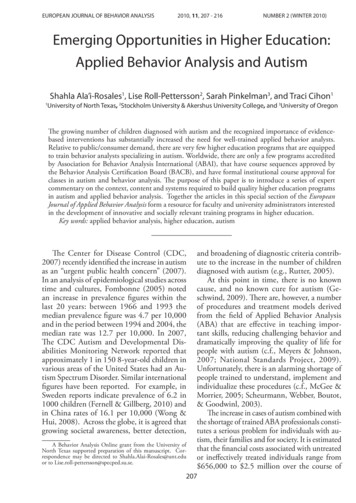
822.2System DescriptionBurner systemThe burner system had a separate control system consisting of PI-controllers. Thenumber of burners vary between sections, e.g. in zone 1 Mid the PI-control controls four burners and in zone 2 West it was only one burner. The controlledburners had two modes either on or off. Since the burners only operated withtwo modes the control signal was converted to a burning time for the burners.The PI-controllers were implemented as series PI-controllers.F(s) K(1 I 1)s1The parameters were K 3.36 and I 93.46. The burning time was given bythe cycle time multiplied by the control signal and the numbers of burners in thesection. To minimize the frequency of switching between on and off the burningtime was set to zero if it was less than 5 seconds and to maximum burning time ifit was greater than maximum burning time minus 10 seconds. The burner systemcan be summarized in the following algorithm:Algorithm for burner system:1. Wait until a cycle time have passed.2. Calculate the burn time as the cycle time multiplied withthe controlsignal and the number of burners in the section.3. If the burn time is less than 5 seconds set it to zero.4. If the burn time is greater than maximum burn time minus 10 seconds set it to maximum burn time.5. Set the next burner to burn for the burn time.6. Update next burner, whose burning time shall be calculated the nexttime, to the last burner to have it burn time set.7. Repeat from step one.If a section had two burners and the control signal was 50 %, the burnersburned on each half of the time, or if there were two burners with the signal 25% half of the time no burner would burn. Figure 2.3 shows the burner systemfor section 2, which has 4 burners, with the control signal at 25 %, the burnersoperates in series, when the first one is done the next starts and so on. Figure 2.4shows the same section for 60%, the burner are now working more in parallel. Inthe system today none of the burners in zone 1 and 2 east are on since it is alreadyto hot there. There is small delay before the burner starts to burn.

Burner 12.29Burner 0300350250300350Burner 21.510.50-0.5Burner r 4Time1.510.50-0.5050100150200TimeFigure 2.3: How the burner system act with an input of 25%, a one representthat the burner is on and a zero that it is off.

10Burner 11.510.50-0.5Burner 221.510.50-0.5050100150200System e050100150200Burner 31.510.50-0.5Burner igure 2.4: How the burner system act with an input of 60%, one representthat the burner is on and zero that it is off.

3Control design theoryThe purpose of this chapter is to give the background for the different controldesigns that were implemented in this thesis. The different controllers that wereused were split range control, MPC and DMPC.3.1Split range controlSplit range control is a simple control strategy which can be used when there aremore than one input that controls the same output. The basic idea is to dividethe control signal into different ranges for the input signals. In the case of twoburners, only one will burn in the range 0-50 % and the other is off, and in therange 50-100 % one will burn all the time and the other is burning according tothe control signal. A setup for a system with a split range controller can be seenin Figure 3.1u1reftempPI-Control%Burner 1Split-rangeu2Burner 2Figure 3.1: A sketch for the setup of the system with the split range controller implemented.A split range control can decrease frequency the burners turn on and off since11

123Control design theoryall the burners in a section, except one is burning at 100 or 0 %. The split rangecontrol have two parameters, swap time and cycle time. Swap time decides thetime between the swap of the range for the burners. The burners have differentpositions inside the section, and therefore affect the temperature in its own section and nearby sections differently.The use of swap time is to minimize the effect of the burners position such asuneven temperature within the section. The cycle time is used in the same wayas in the current burner system, i.e., to convert the control signal to a burn timeby multiplying the control signal with the cycle time. An example of the signalfrom the burners can be seen in Figure 3.2. The split range controller can besummarized with the following algorithm:Algorithm for split range:1. Wait until it is time to calculate the burn time.2. If the time that has passed since the last swap is greater than theswap time. Change the operating range for the burners.3. Calculate and set the burn time for each burner.4. Repeat from step one.

13Model Predictive controlBurner 13.21.510.50 0250300350Burner 2Time1.510.50 0.5050100150Burner 3Time1.510.50 0.5050100150Burner 4Time1.510.50 0.5050100150TimeFigure 3.2: This shows how the burners act when the split range controllerhave an input signal of 60 %, 1 represent that the burner is on and 0 that isoff.3.2Model Predictive controlIn this section the MPC is introduced. We first present the background and a basic MPC formulation. An advantage of the MPC is its flexibility and that the basicformulation can be extended to include reference tracking, feedforward controland relaxed constraints, as described. For further reading see [6].3.2.1BackgroundModel predictive control is based on solving an optimization problem for eachsample instant. The solution to the optimization problem is a sequence of controlsignals to be used now and in the future. Of the sequence of control signals,only the first is applied to the controlled system and the rest is discarded. Thisprocedure is repeated for each sample instant and achieves a feedback controlas the optimization problem is performed when new measurements are madeavailable. If the whole sequence would be applied it would be open loop control.The model of the controlled system is a part of the optimization problem and isused to predict the future states. The MPC can be seen as it performing an openloop optimization for each sample instant.

1433.2.2Control design theoryDescription of the model predictive controllerThis section will introduce the model predictive controller with a theoretical example. The objective for the MPC is to bring the system states and the input tozero, subject to the system dynamics and limitations. In the basic setup the costfunction is quadratic and the constraints are linear.minimizeu( · )NX x(k j) 2Q1 u(k j 1) 2Q2j 1subject to(3.1)x(k i) Ax(k i) Bu(k i)xmin xi xmaxumin ui umaxHere N represents the prediction horizon which determine how many steps forward the controller predicts. The norm x 2Q is the euclidean norm weighted bythe weight matrix Q, x T Qx. The difference between the weight matrices Q1 andQ2 determinate the behaviour for the controller. If Q1 is large in comparison toQ2 will the system states will converge to zero fast, at the cost of large controlinputs. If Q1 is small in comparison to Q2 will the control inputs be small, at thecost of that, the system states will converge to zero slow.The equality constraints represent the system dynamics from the model of thecontrolled system. The inequality constraints are bounds for the system statesand/or the control signal, which are typically for safety regulations or saturation.In summary the MPC can be explained by the following algorithm:Algorithm for MPC:1. Measure the system state x(k)2. Compute the control signal sequence u( · ) for the problem in (3.1)3. Use the first element u(k) in the sequence from the previous stepduring one sample4. Time update, k k 15. Repeat from step 1

3.215Model Predictive control3.2.3Reference TrackingIn the formulation in (3.1) the system will be driven to a steady state at the origin.In order to steer the system to any other state than the origin, the MPC formulation must be extended to include reference tracking. This can partially be accomplished by minimizing the difference between a state and reference. This gives aa conflict in the MPC formulation which is to have the states follow a referenceand try to keep the input zero. One solution is to minimize the increment of theinput signals instead of its amplitude. The reformulation (3.2) gives the MPCcontroller reference tracking.minimizeu( · )NX x(k j) r(k j) 2Q1 u(k j 1) u(k j 2) 2Q2j 1subject tox(k i) Ax(k i) Bu(k i)(3.2)xmin xi xmaxumin ui umax3.2.4Feedforward ControlIn feedforward control the disturbance is measured and with used in the controlcomputation to remove some of the disturbance effect on the system. It thus hasan advantage compared to feedback control which has to wait for the disturbanceto effect the system before it can take suitable action. The effectiveness of feedforward control is limited by the model of the measurable disturbance to the output,and any remaining unmeasurable disturbances. Therefore feedforward controlis implemented together with feedback control. The feedforward control part removes most of the measurable disturbance effect and feedback control take careof the rest and also any unmeasured disturbance. Feedforward control is implemented in MPC by including the disturbance effect in the predicted future outputs, which can be seen in (3.3). The optimizer then accounts for the disturbancewhen it computes the control signal.

163minimizeu( · )NXControl design theory x(k j) 2Q1 u(k j 1) 2Q2j 1subject tox(k i) Ax(k i) Bu(k i) Bd dm (k i)(3.3)xmin xi xmaxumin ui umax3.2.5Relaxed ConstraintsA serious problem for the MPC is when the optimization problem is infeasible.This can happen because an unexpected large disturbance occurred and it is impossible for the controller to prevent that a state breaks its constraint. Thereforeit is important that the MPC controller has a strategy to handle infeasible problem. A systematic strategy is to make relaxed constraints which can be broken ifthere is no admissible solution [6]. The constraints on the input signal are usually"hard" and cannot be broken since it commonly represent a physical limitationon the actuator. Therefore it is usually the constraints on the output which arerelaxed.A constraint is relaxed by introducing a new variable which is non-zero whenthe constraint is violated. Such a variable is called slack variable. To avoid violation of constraints when unnecessary, a penalty term is added to the objective inorder to try to obtain a zero slack. The optimization problem then becomesminimizeu( · )NX x(k j) 2Q1 u(k j 1) 2Q2 λ j 1subject tox(k i) Ax(k i) Bu(k i)(3.4)xmin xi xmax umin ui umax0 The reason for not using the euclidean norm on in the cost function is thatall active constraint will be violated for all finite λ, even when it is not necessary.From the true constrained x there exist a move to an infeasible solution x d for some vector d which will decrease the cost with O( ). With the euclidean

3.317DMPCnorm will the cost of violating the constraint be O( 2 ) which gives a net reduction in the cost for small . With the 1-norm in the cost function a sufficient λwill ensure that violation occur only when the original problem is infeasible.3.2.6Complete modelThe different modifications of the basic formulation can be used together andgives the following optimization problem, which will be the form used later.minimizeu( · )NX x(k j) r(k j) 2Q1 u(k j 1) u(k j 2) 2Q2 λ j 1subject tox(k i) Ax(k i) Bu(k i) Bd dm (k i)(3.5)xmin xi xmax umin ui umax0 3.3DMPCAnother way to use the function of MPC is to enlarge the system with more MPCcontrollers. This type of control strategy is called distributed model predictivecontrol. The meaning of DMPC is to split the problem into sub systems, whereevery MPC controller computes a control input locally. This will make it easierfor the solver, as the optimization problems will be smaller. However, when doing this, the interaction between the different controllers and parts of the systemswill not be part of the models used locally in every MPC controller. One approximation, which we will use, is to assume that the states from other zones will beconstant over the prediction horizon. For further reading about DMPC, see [9].

4Model estimationThis chapter is about the identification and validation of the model for the systemdescribed in Chapter 2. The workflow for the model estimation was an iterativeprocess; it started with a simple model that was extended until no improvementscould be found. The main idea with the model was to keep it simple with relevant relations, which capture the dominant behaviour of the system.4.1Black-box modellingThere are three different approaches of deriving models; White-box, Grey-boxand Black-box. The White-box model is based only on known information aboutthe system. If all information about the system is known and the model has theright structure, the model and the system will be identical. In the case of the furnace much of the information is missing, such as the heat transfer between thesections and heat losses through the walls. It could be possible to model thoserelations based on thermodynamics, but many parameters are unknown such asthe flow of the flue gas and need to be estimated. A White-box model of the furnace would be very complex and some relations are hard to describe with physics.For example the temperatures zig-zag behaviour caused by the walking beam.The advantage with a Black-box model is that it can be used when no information about the system is known. The Black-box model describes the relationsbetween the input and output signals without having a structure based on physical relations of the system.

Three different control strategies were applied, Split range, model predictive con-trol (MPC) and distributed model predictive control (DMPC). The MPC prob-lems were formulated by using the toolbox YALMIP [5] and were solved with the solver MOSEK [2]. All strategies were then evaluated, in terms of temperature and numbers of switches for the .