WIXLIB

1The foundations of calculus of variationsThe problem of the calculus of variations evolves from the analysis of functions. In the analysis of functions the focus is on the relation between twosets of numbers, the independent (x) and the dependent (y) set. The function f creates a one-to-one correspondence between these two sets, denoted asy f (x).The generalization of this concept is based on allowing the two sets not beingrestricted to be real numbers and to be functions themselves. The relationship between these sets is now called a functional. The topic of the calculusof variations is to find extrema of functionals, most commonly formulated inthe form of an integral.1.1The fundamental problem and lemma of calculus ofvariationsThe fundamental problem of the calculus of variations is to find the extremum(maximum or minimum) of the functionalZ x1I(y) f (x, y, y 0 )dx,x0where the solution satisfies the boundary conditionsy(x0 ) y0andy(x1 ) y1 .This problem may be generalized to the cases when higher derivatives or multiple functions are given and will be discussed in Chapters 3 and 4, respectively.These problems may also be extended with constraints, the topic of Chapter 2.A solution process may be arrived at with the following logic. Let us assume that there exists such a solution y(x) for the above problem that satisfies3

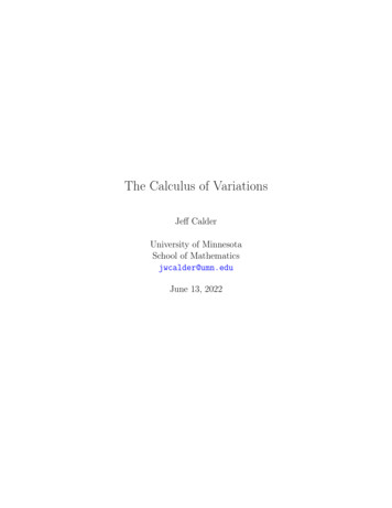
4Applied calculus of variations for engineersthe boundary conditions and produces the extremum of the functional. Furthermore, we assume that it is twice differentiable. In order to prove thatthis function results in an extremum, we need to prove that any alternativefunction does not attain the extremum.We introduce an alternative solution function of the formY (x) y(x) η(x),where η(x) is an arbitrary auxiliary function of x, that is also twice differentiable and vanishes at the boundary:η(x0 ) η(x1 ) 0.In consequence the following is also true:Y (x0 ) y(x0 ) y0andY (x1 ) y(x1 ) y1 .A typical relationship between these functions is shown in Figure 1.1 wherethe function is represented by the solid line and the alternative function bythe dotted line. The dashed line represents the arbitrary auxiliary function.Since the alternative function Y (x) also satisfies the boundary conditionsof the functional, we may substitute into the variational problem.Z x1f (x, Y, Y 0 )dx.I( ) x0whereY 0 (x) y 0 (x) η 0 (x).The new functional in terms of is identical with the original in the case when 0 and has its extremum when I( ) 0 0. Executing the derivation and taking the derivative into the integral, since thelimits are fixed, with the chain rule we obtainZ x1 I( ) f dY f dY 0 ( )dx. Y 0 d x0 Y d ClearlydY η(x),d

5The foundations of calculus of 40.60.81FIGURE 1.1 Alternative solutions exampleanddY 0 η 0 (x),d resulting in I( ) Zx1(x0 f f 0η(x) η (x))dx. Y Y 0Integrating the second term by parts yieldsZ x1Z x1 f 0 fd fx1(η (x))dx η(x) x0 ()η(x)dx.000 Yx0 Yx0 dx YDue to the boundary conditions, the first term vanishes. With substitutionand factoring the auxiliary function, the problem becomesZ x1 I( ) fd f ( )η(x)dx. dx Y 0x0 YThe extremum is achieved when 0 as stated above, henceZ x1 I( ) fd f 0 ( )η(x)dx. ydx y 0x0

6Applied calculus of variations for engineersLet us now consider the following integral:Zx1η(x)F (x)dx,x0where x0 x x1 and F (x) is continuous, while η(x) is continuously differentiable, satisfyingη(x0 ) η(x1 ) 0.The fundamental lemma of calculus of variations states that if for all such η(x)Zx1η(x)F (x)dx 0,x0thenF (x) 0in the whole interval.The following proof by contradiction is from [13]. Let us assume that thereexists at least one such location x0 ζ x1 where F (x) is not zero, forexampleF (ζ) 0.By the condition of continuity of F (x) there must be a neighborhood ofζ h ζ ζ hwhere F (x) 0. In this case, however, the integral becomesZx1η(x)F (x)dx 0,x0for the right choice of η(x), which contradicts the original assumption. Hencethe statement of the lemma must be true.Applying the lemma to this case results in the Euler-Lagrange differential equation specifying the extremum fd f 0. ydx y 0

The foundations of calculus of variations1.27The Legendre testThe Euler-Lagrange differential equation just introduced represents a necessary, but not sufficient, condition for the solution of the fundamental variational problem.The alternative functional ofI( ) Zx1f (x, Y, Y 0 )dx,x0may be expanded asZI( ) x1f (x, y η(x), y 0 η 0 (x))dx.x0Assuming that the f function has continuous partial derivatives, the meanvalue theorem is applicable:f (x, y η(x), y 0 η 0 (x)) f (x, y, y 0 ) (η(x) f (x, y, y 0 ) f (x, y, y 0 ) η 0 (x)) O( 2 ). y y 0By substituting we obtainI( ) Z x1(η(x)x0Zx1f (x, y, y 0 )dx x0 f (x, y, y 0 ) f (x, y, y 0 ) η 0 (x))dx O( 2 ). y y 0With the introduction ofδI1 Zx1(η(x)x0 f (x, y, y 0 ) f (x, y, y 0 ) η 0 (x))dx, y y 0we can writeI( ) I(0) δI1 O( 2 ),where δI1 is called the first variation. The vanishing of the first variation is anecessary, but not sufficient, condition to have an extremum. To establish asufficient condition, assuming that the function is thrice continuously differentiable, we further expand asI( ) I(0) δI1 δI2 O( 3 ).

8Applied calculus of variations for engineersHere the newly introduced second variation is 2δI2 2Zx1(η 2 (x)x02η(x)η 0 (x)η 02 (x) 2 f (x, y, y 0 ) y 2 2 f (x, y, y 0 ) y y 0 2 f (x, y, y 0 ))dx. y 02We now possess all the components to test for the existence of the extremum(maximum or minimum). The Legendre test in [5] states that if independently of the choice of the auxiliary η(x) function- the Euler-Lagrange equation is satisfied,- the first variation vanishes (δI1 0), and- the second variation does not vanish (δI2 6 0)over the interval of integration, then the functional has an extremum. Thistest manifests the necessary conditions for the existence of the extremum.Specifically, the extremum will be a maximum if the second variation is negative, and conversely a minimum if it is positive. Certain similarities to theextremum evaluation of regular functions by the teaching of classical calculusare obvious.We finally introduce the variation of the function asδy Y (x) y(x) η(x),and the variation of the derivative asδy 0 Y 0 (x) y 0 (x) η 0 (x).Based on these variations, we distinguish between the following cases:- strong extremum occurs when δy is small, however, δy 0 is large, while- weak extremum occurs when both δy and δy 0 are small.On a final note: the above considerations did not ever state the finding orpresence of an absolute extremum; only the local extremum in the interval ofthe integrand is obtained.

The foundations of calculus of variations1.39The Euler-Lagrange differential equationLet us expand the derivative in the second term of the Euler-Lagrange differential equation as follows:d f 2f 2 f 0 2 f 00 y 02 y .00dx y x y y y 0 yThis demonstrates that the Euler-Lagrange equation is usually of second order. f 2f 2 f 0 2 f 00 y 02 y 0. y x y 0 y y 0 yThe above form is also called the extended form. Consider the case when themultiplier of the second derivative term vanishes: 2f 0. y 02In this case f must be a linear function of y 0 , in the form off (x, y, y 0 ) p(x, y) q(x, y)y 0 .For this form, the other derivatives of the equation are computed as f p q 0 y, y y y f q, y 0 2f q ,0 x y xand 2f q . y y 0 ySubstituting results in the Euler-Lagrange differential equation of the form p q 0, y xor p q . y xIn order to have a solution, this must be an identity, in which case there mustbe a function of two variablesu(x, y)

10Applied calculus of variations for engineerswhose total differential is of the formdu p(x, y)dx q(x, y)dy f (x, y, y 0 )dx.The functional may be evaluated asI(y) Zx10f (x, y, y )dx x0Zx1x0du u(x1 , y1 ) u(x0 , y0 ).It follows from this that the necessary and sufficient condition for the solution of the Euler-Lagrange differential equation is that the integrand of thefunctional be the total differential with respect to x of a certain function ofboth x and y.Considering furthermore, that the Euler-Lagrange differential equation islinear with respect to f , it also follows that a term added to f will not changethe necessity and sufficiency of that condition.Another special case may be worthy of consideration. Let us assume thatthe integrand does not explicitly contain the x term. Then by executing thedifferentiationsd 0 f(y f) dx y 0y0d f f f 0 y dx y 0 x yy0 (d f f f ) .0dx y y xWith the last term vanishing in this case, the differential equation simplifies tod 0 f(y f ) 0.dx y 0Its consequence is the expression also known as Beltrami’s formula:y0 f f c1 , y 0(1.1)where the right-hand side term is an integration constant. The classical problem of the brachistochrone, discussed in the next section, belongs to this class.Finally, it is also often the case that the integrand does not contain the yterm explicitly. Then f 0 y

The foundations of calculus of variations11and the differential equation has the simplerd f 0dx y 0form. As above, the result is f c2 y 0where c2 is another integration constant. The geodesic problems, also thesubject of Chapter 7, represent this type of Euler-Lagrange equations.We can surmise that the Euler-Lagrange differential equation’s general solution is of the formy y(x, c1 , c2 ),where the c1 , c2 are constants of integration, and are solved from the boundary conditionsy0 y(x0 , c1 , c2 )andy1 y(x1 , c1 , c2 ).1.4Application: Minimal path problemsThis section deals with several classical problems to illustrate the methodology. The problem of finding the minimal path between two points in spacewill be addressed in different senses.The first problem is simple geometry, the shortest geometric distance between the points. The second one is the well-known classical problem of thebrachistochrone, originally posed and solved by Bernoulli. This is the pathof the shortest time required to move from one point to the other under theforce of gravity.The third problem considers a minimal path in an optical sense and leadsto Snell’s law of reflection in optics. The fourth example finds the path ofminimal kinetic energy of a particle moving under the force of gravity.All four problems will be presented in two-dimensional space, although theymay also be posed and solved in three dimensions with some more algebraicdifficulty but without any additional instructional benefit.

12Applied calculus of variations for engineers1.4.1Shortest curve between two pointsFirst we consider the rather trivial variational problem of finding the solutionof the shortest curve between two points, P0 , P1 , in the plane. The form ofthe problem using the arclength expression isZP1ds P0Zx1x0p1 y 02 dx extremum.The obvious boundary conditions are the curve going through its endpoints:y(x0 ) y0 ,andy(x1 ) y1 .It is common knowledge that the solution in Euclidean geometry is a straightline from point (x0 , y0 ) to point (x1 , y1 ). The solution function is of the formy(x) y0 m(x x0 ),with slopem y1 y 0.x1 x 0To evaluate the integral, we compute the derivative asy0 mand the function becomesf (x, y, y 0 ) p1 m2 .Since the integrand is constant, the integral is trivialZ x1ppI(y) 1 m2dx 1 m2 (x1 x0 ).x0The square of the functional isI 2 (y) (1 m2 )(x1 x0 )2 (x1 x0 )2 (y1 y0 )2 .This is the square of the distance between the two points in plane, hencethe extremum is the distance between the two points along the straight line.Despite the simplicity of the example, the connection of a geometric problemto a variational formulation of a functional is clearly visible. This will be themost powerful justification for the use of this technique.Let us now solve theZx1x0p1 y 02 dx extremum

The foundations of calculus of variations13problem via its Euler-Lagrange equation form. Note that the form of the integrand dictates the use of the extended form. f 0, y 2f 0, x y 0 2f 0, y y 0and 2f1 . y 02(1 y 02 )3/2Substituting into the extended form gives1y 00 0,(1 y 02 )3/2which simplifies intoy 00 0.Integrating twice, one obtainsy(x) c0 c1 x,clearly the equation of a line. Substituting into the boundary conditions weobtain two equations,y 0 c 0 c 1 x0 ,andy 1 c 0 c 1 x1 .The solution of the resulting linear system of equations isc 0 y 0 c 1 x0 ,andc1 It is easy to reconcile thaty(x) y0 is identical toy1 y 0.x1 x 0y1 y 0y1 y 0x0 xx1 x 0x1 x 0y(x) y0 m(x x0 ).

14Applied calculus of variations for engineersThe noticeable difference between the two solutions of this problem is thatusing the Euler-Lagrange equation required no a priori assumption on theshape of the curve and the geometric know-how was not used. This is thecase in most practical engineering applications and this is the reason for theutmost importance of the Euler-Lagrange equation.1.4.2The brachistochrone problemThe problem of the brachistochrone may be the first problem of variationalcalculus, already solved by Johann Bernoulli in the late 1600s. The namestands for the shortest time in Greek, indicating the origin of the problem.The problem is elementary in a physical sense. Its goal is to find the shortestpath of a particle moving in a vertical plane from a higher point to a lowerpoint under the (only) force of gravity. The sought solution is the functiony(x) with boundary conditions y(x0 ) y0 and y(x1 ) y1 whereP0 (x0 , y0 )andP1 (x1 , y1 )are the starting and terminal points, respectively. Based on elementary physicsconsiderations, the problem represents an exchange of potential energy withkinetic energy.A moving body’s kinetic energy is related to its velocity and its mass. Thehigher the velocity and the mass, the bigger the kinetic energy. A body cangain kinetic energy using its potential energy, and conversely, can use its kinetic energy to build up potential energy. At any point during the movement,the total energy is at equilibrium. This is the principle of Hamilton’s thatwill be discussed in more detail in Chapter 9.The potential energy of the particle at any x, y point during the motion isEp mg(y0 y),where m is the mass of the particle and g is the acceleration of gravity. Thekinetic energy is1mv 22assuming that the particle at the (x, y) point has velocity v. They are inbalance asEk Ek E p ,

15The foundations of calculus of variationsresulting in an expression of the velocity asv The velocity by definition isp2g(y0 y).v ds,dtwhere s is the arclength of the yet unknown curve. The time required to runthe length of the curve ist ZP1dt P0ZP1P01ds.vUsing the arclength expression from calculus, we getZ x1 1 y02t dx.vx0Substituting the velocity expression yieldsZ x1 11 y02 t dx.y0 y2g x0Since we are looking for the minimal time, this is a variational problem of1I(y) 2gZx1x0 1 y02 dx extremum.y0 yThe integrand does not contain the independent variable, hence we can applyBeltrami’s formula of equation (1.1). This results in the form ofpy 021 y 02p c0 .y0 y(y0 y)(1 y 02 )Creating a common denominator on the left-hand side producespp y 02 y0 y 1 y 02 (y0 y)(1 y 02 )p c0 . (y0 y)(1 y 02 ) y0 yGrouping the numerator simplifies to y0 yp c0 . (y0 y)(1 y 02 ) y0 yCanceling and squaring results in the solution for y 0 asy 02 1 c20 (y0 y).c20 (y0 y)

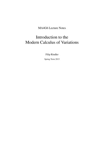
16Applied calculus of variations for engineersSincedy 2) ,dxthe differential equation may be separated as y0 ydx pdy.2c1 (y0 y)y 02 (Here the new constant is introduced for simplicity asc1 1.2c20Finally x may be expressed directly by integrating Zy0 ypx dy c2 .2c1 (y0 y)The usual trigonometric substitution ofty0 y 2c1 sin2 ( )2yields the integral ofx 2c1Ztsin2 ( )dt c1 (t sin(t)) c2 ,2where c2 is another constant of integration. Reorganizing yieldsy y0 c1 (1 cos(t)).The final solution of the brachistochrone problem therefore is a cycloid. Figure 1.2 depicts the problem of the point moving from (0, 1) until it reachesthe x axis.The resulting curve seems somewhat counter-intuitive, especially in view ofthe earlier example of the shortest geometric distance between two points inthe plane and demonstrated by the straight line chord between the two points.The shortest time, however, when the speed obtained during the traversal ofthe interval depends on the path taken, is an entirely different matter.The constants of the integration may be solved by substituting the boundary points. From the x equation above at t 0 we easily findx c 2 x0 .Substituting the endpoint location into the y equation, we obtainy y0 c1 (1 cos(t)) y1 ,

17The foundations of calculus of variations1x(t), 6FIGURE 1.2 Solution of the brachistochrone problemwhich is inconclusive, since the time of reaching the endpoint is not known.For a simple conclusion of this discussion, let us assume that the particlereaches the endpoint at time t Π/2. Thenc1 y 0 y 1 ,and the final solution isx x0 (y0 y1 )(t sin(t))andy y1 (1 cos(t)).For the case shown in Figure 1.2, the point moving from (0, 1) until it reachesthe x axis, the solution curve isx (t sin(t))andy cos(t).Another intriguing characteristic of the brachistochrone particle is thatwhen two particles are let go from two different points of the curve they will

18Applied calculus of variations for engineersreach the terminal point of the curve at the same time. This is also counterintuitive, since clearly they have different geometric distances to cover; however, since they are acting under the gravity and the slope of the curve isdifferent at the two locations, the particle starting from a higher locationgathers much bigger speed than the particle starting at a lower location.This, so-called tautochrone, behavior may be proven by calculation of thetime of the particles using the formula developed earlier. Evaluation of thisintegral between points (x0 , y0 ) and (x1 , y1 ) as well as between (x2 , y2 ) and(x1 , y1 ) (where (x2 , y2 ) lies on the solution curve anywhere between the starting and terminal point) will result in the same time.Hence the brachistochrone problem may also be posed with a specified terminal point and a variable starting point, leading to the class of variationalproblems with open boundary, subject of Section 1.5.1.4.3Fermat’s principleFermat’s principle states that light traveling through an inhomogeneous mediumchooses the path of minimal optical length. The path’s optimal length dependson the speed of light in th

With the emphasis on applications, the second part starts with a detailed discussion of the geodesic concept of di erential geometry and its extensions to higher order spaces. The computational geometry chapter covers the vari-ational origin of natural splines and the variational formulation of B-splines under various constraints.