Transcription
MA4G6 Lecture NotesIntroduction to theModern Calculus of VariationsFilip RindlerSpring Term 2015
Filip RindlerMathematics InstituteUniversity of WarwickCoventry CV4 7ALUnited c.uk/filiprindlerCopyright 2015 Filip Rindler.Version 1.1.
PrefaceThese lecture notes, written for the MA4G6 Calculus of Variations course at the Universityof Warwick, intend to give a modern introduction to the Calculus of Variations. I have triedto cover different aspects of the field and to explain how they fit into the “big picture”.This is not an encyclopedic work; many important results are omitted and sometimes Ionly present a special case of a more general theorem. I have, however, tried to strike abalance between a pure introduction and a text that can be used for later revision of forgottenmaterial.The presentation is based around a few principles: The presentation is quite “modern” in that I use several techniques which are perhapsnot usually found in an introductory text or that have only recently been developed. For most results, I try to use “reasonable” assumptions, not necessarily minimal ones. When presented with a choice of how to prove a result, I have usually preferred the(in my opinion) most conceptually clear approach over more “elementary” ones. Forexample, I use Young measures in many instances, even though this comes at theexpense of a higher initial burden of abstract theory. Wherever possible, I first present an abstract result for general functionals defined onBanach spaces to illustrate the general structure of a certain result. Only then do Ispecialize to the case of integral functionals on Sobolev spaces. I do not attempt to trace every result to its original source as many results have evolvedover generations of mathematicians. Some pointers to further literature are given inthe last section of every chapter.Comment.Most of what I present here is not original, I learned it from my teachers and colleagues, both through formal lectures and through informal discussions. Published worksthat influenced this course were the lecture notes on microstructure by S. Müller [73], theencyclopedic work on the Calculus of Variations by B. Dacorogna [25], the book on Youngmeasures by P. Pedregal [81], Giusti’s more regularity theory-focused introduction to theCalculus of Variations [44], as well as lecture notes on several related courses by J. Ball,J. Kristensen, A. Mielke. Further texts on the Calculus of Variations are the elementaryintroductions by B. van Brunt [96] and B. Dacorogna [26], the more classical two-part treatise [39, 40] by M. Giaquinta & S. Hildebrandt, as well as the comprehensive treatment of
iiPREFACEthe geometric measure theory aspects of the Calculus of Variations by Giaquinta, Modica& Souček [41, 42].In particular, I would like to thank Alexander Mielke and Jan Kristensen, who are responsible for my choice of research area. Through their generosity and enthusiasm in sharing their knowledge they have provided me with the foundation for my study and research.Furthermore, I am grateful to Richard Gratwick and the participants of the MA4G6 coursefor many helpful comments, corrections, and remarks.These lecture notes are a living document and I would appreciate comments, correctionsand remarks – however small. They can be sent back to me via e-mail atF.Rindler@warwick.ac.ukor anonymously viahttp://tinyurl.com/MA4G6-2015or by scanning the following QR-Code:Moreover, every page contains its individual QR-code for immediate feedback. I encourageall readers to make use of them.Comment.F. R.January 2015
ContentsPrefaceiContentsiii1 Introduction1.1 The brachistochrone problem . . . . . .1.2 Electrostatics . . . . . . . . . . . . . .1.3 Stationary states in quantum mechanics1.4 Hyperelasticity . . . . . . . . . . . . .1.5 Optimal saving and consumption . . . .1.6 Sailing against the wind . . . . . . . . .12456892 Convexity2.1 The Direct Method . . . . . . . . .2.2 Functionals with convex integrands .2.3 Integrands with u-dependence . . .2.4 The Euler–Lagrange equation . . . .2.5 Regularity of minimizers . . . . . .2.6 Lavrentiev gap phenomenon . . . .2.7 Invariances and the Noether theorem2.8 Side constraints . . . . . . . . . . .2.9 Notes and bibliographical remarks .11121418192431333741.434451546266687374753 Quasiconvexity3.1 Quasiconvexity . . . . . . . . . . . .3.2 Null-Lagrangians . . . . . . . . . . .3.3 Young measures . . . . . . . . . . . .3.4 Gradient Young measures . . . . . . .3.5 Gradient Young measures and rigidity3.6 Lower semicontinuity . . . . . . . . .3.7 Integrands with u-dependence . . . .3.8 Regularity of minimizers . . . . . . .3.9 Notes and bibliographical remarks . .Comment.
iv4 Polyconvexity4.1 Polyconvexity . . . . . . . . . . .4.2 Existence Theorems . . . . . . . .4.3 Global injectivity . . . . . . . . .4.4 Notes and bibliographical remarksCONTENTS.7778798586.5 Relaxation5.1 Quasiconvex envelopes . . . . . . . . . . . .5.2 Relaxation of integral functionals . . . . . . .5.3 Young measure relaxation . . . . . . . . . . .5.4 Characterization of gradient Young measures5.5 Notes and bibliographical remarks . . . . . .87. 88. 91. 95. 101. 105A PrerequisitesA.1 General facts and notation . . . . . . . .A.2 Measure theory . . . . . . . . . . . . . .A.3 Functional analysis . . . . . . . . . . . .A.4 Sobolev and other function spaces phy
Chapter 1IntroductionPhysical modeling is a delicate business – trying to balance the validity of the resultingmodel, that is, its agreement with nature and its predictive capabilities, with the feasibilityof its mathematical treatment is often highly non-straightforward. In this quest to formulatea useful picture of an aspect of the world, it turns out on surprisingly many occasions thatthe formulation of the model becomes clearer, more compact, or more descriptive, if oneintroduces some form of a variational principle, that is, if one can define a quantity, such asenergy or entropy, which obeys a minimization, maximization or saddle-point law.How “fundamental” such a scalar quantity is perceived depends on the situation: Forexample, in classical mechanics, one calls forces conservative if they can be expressed asthe derivative of an “energy potential” along a curve. It turns out that many, if not most,forces in physics are conservative, which seems to imply that the concept of energy is fundamental. Furthermore, Einstein’s famous formula E mc2 expresses the equivalence ofmass and energy, positioning energy as the “most” fundamental quantity, with mass becoming “condensed” energy. On the other hand, the other ubiquitous scalar physical quantity,the entropy, has a more “artificial” flavor as a measure of missing information in a model,as is now well understood in Statistical Mechanics, where entropy becomes a derived quantity. We leave it to the field of Philosophy of Science to understand the nature of variationalconcepts. In the words of William Thomson, the Lord Kelvin1 :The fact that mathematics does such a good job of describing the Universe isa mystery that we don’t understand. And a debt that we will probably never beable to repay.Our approach to variational quantities here is a pragmatic one: We see them as providingstructure to a problem and to enable different mathematical, so-called variational, methods.For instance, in elasticity theory it is usually unrealistic that a system will tend to a globalminimizer by itself, but this does not mean that – as an approximation – such a principlecannot be useful in practice. On a fundamental level, there probably is no minimization assuch in physics, only quantum-mechanical interactions (or whatever lies “below” quantumprove nothing, however. Thomson also said “X-rays will prove to be a hoax”.Comment.1 Quotes
2CHAPTER 1. INTRODUCTIONmechanics). However, if we wait long enough, the inherent noise in a realistic system willmove our system around and it will settle with a high probability in a low-energy state.In this course, we will focus solely on minimization problems for integral functionalsof the form (Ω Rd open and bounded) Ωf (x, u(x), u(x)) dx min,u : Ω Rm ,possibly under conditions on the boundary values of u and further side constraints. Theseproblems form the original core of the Calculus of Variations and are as relevant today asthey have always been. The systematic understanding of these integral functionals startsin Euler’s and Bernoulli’s times in the late 1600s and the early 1700s, and their studywas boosted into the modern age by Hilbert’s 19th, 20th, 23rd problems, formulated in1900 [47]. The excitement has never stopped since and new and important discoveries aremade every year.We start this course by looking at a parade of examples, which we treat at varying levelsof detail. All these problems will be investigated further along the course once we havedeveloped the necessary mathematical tools.1.1 The brachistochrone problemIn June 1696 Johann Bernoulli published a problem in the journal Acta Eruditorum, whichcan be seen as the time of birth of the Calculus of Variations (the name, however, is fromLeonhard Euler’s 1766 treatise Elementa calculi variationum). Additionally, Bernoulli senta letter containing the question to Gottfried Wilhelm Leibniz on 9 June 1696, who returnedhis solution only a few days later on 16 June, and commented that the problem tempted him“like the apple tempted Eve” because of its beauty. Isaac Newton published a solution (afterthe problem had reached him) without giving his identity, but Bernoulli identified him “exungue leonem” (from Latin, “by the lion’s claw”). The problem was formulated as follows2 :Given two points A and B in a vertical [meaning “not horizontal”] plane, oneshall find a curve AMB for a movable point M, on which it travels from A to Bin the shortest time, only driven by its own weight.The resulting curve is called the brachistochrone (from Ancient Greek, “shortest time”)curve.We formulate the problem as follows: We look for the curve y connecting the origin(0, 0) to the point (x̄, ȳ), where x̄ 0, ȳ 0, such that a point mass m 0 slides from restat (0, 0) to (x̄, ȳ) quickest among all such curves. See Figure 1.1 for several possible slidepaths. We parametrize a point (x, y) on the curve by the time t 0. The point mass hasComment.2 The German original reads “Wenn in einer verticalen Ebene zwei Punkte A und B gegeben sind, sollman dem beweglichen Punkte M eine Bahn AMB anweisen, auf welcher er von A ausgehend vermöge seinereigenen Schwere in kürzester Zeit nach B gelangt.”
1.1. THE BRACHISTOCHRONE PROBLEM3Figure 1.1: Several slide curves from the origin to (x̄, ȳ).kinetic and potential energies{( )2 ( )2 }( ) {( )2 }dxdym dx 2dym 1 ,Ekin 2dtdt2 dtdxEpot mgy,where g 9.81 m/s2 is the (constant) gravitational acceleration on Earth. The total energyEkin Epot is zero at the beginning and conserved along the path. Hence, for all y we have( ) {( )2 }m dx 2dy1 mgy.2 dtdxWe can solve this for dt/dx (where t t(x) is the inverse of the x-parametrization) to get ()dt1 (y′ )2dt 0 ,dx 2gydxdywhere we wrote y′ dx. Integrating over the whole x-length along the curve from 0 to x̄,we get for the total time duration T [y] that x̄11 (y′ )2T [y] dx. y2g 0Comment.We may drop the constant in front of the integral, which does not influence the minimizationproblem, and set x̄ 1 by reparametrization, to arrive at the problem 1 1 (y′ )2 F [y] : dx min, y0 y(0) 0, y(1) ȳ 0.
4CHAPTER 1. INTRODUCTIONClearly, the integrand is convex in y′ , which will be important for the solution theory. Wewill come back to this problem in Example 2.34.A related problem concerns Fermat’s Principle expressing that light (in vacuum or in amedium) always takes the fastest path between two points, from which many optical laws,e.g. about reflection and refraction, can be derived.1.2 ElectrostaticsConsider an electric charge density ρ : R3 R (in units of C/m3 ) in three-dimensionalvacuum. Let E : R3 R3 (in V/m) and B : R3 R3 (in T Vs/m2 ) be the electric andmagnetic fields, respectively, which we assume to be constant in time (hence electrostatics).Assuming that R3 is a linear, homogeneous, isotropic electric material, the Gauss law forelectricity reads · E div E ρ,ε0where ε0 8.854 · 10 12 C/(Vm). Moreover, we have the Faraday law of induction E curl E dB 0.dtThus, since E is curl-free, there exist an electric potential φ : R3 R (in V) such thatE φ .Combining this with the Gauss law, we arrive at the Poisson equation, φ · [ φ ] ρ.ε0(1.1)We can also look at electrostatics in a variational way: We use the norming conditionφ (0) 0. Then, the electric potential energy UE (x; q) of a point charge q 0 (in C) at pointx R3 in the electric field E is given by the path integral (which does not depend on thepath chosen since E is a gradient)UE (x; q) x0qE · ds 10qE(hx) dh qφ (x).Thus, the total electric energy of our charge distribution ρ is (the factor 1/2 is necessary tocount mutual reaction forces correctly)1UE : 2 ε0ρφ dx 32R R3( · E)φ dx,which has units of CV J. Using ( · E)φ · (E φ ) E · ( φ ), the divergence theorem,and the natural assumption that φ vanishes at infinity, we get furtherComment.UE ε02 R3 · (E φ ) E · ( φ ) dx ε02 R3E · ( φ ) dx ε02 R3 φ 2 dx.
1.3. STATIONARY STATES IN QUANTUM MECHANICS5 The integral Ω φ 2 dx is called Dirichlet integral.In Example 2.15 we will see that (1.1) is equivalent to the minimization problem ε0 φ 2 ρφ dx min .2The second term is the energy stored in the electric field caused by its interaction with thecharge density ρ .UE R3ρφ dx R31.3 Stationary states in quantum mechanicsThe non-relativistic evolution of a quantum mechanical system with N degrees of freedomin an electrical field is described completely through its wave function Ψ : RN R Cthat satisfies the Schrödinger equation[] h̄dih̄ Ψ(x,t) V (x,t) Ψ(x,t),x RN , t R,dt2µwhere h̄ 1.05 · 10 34 Js is the reduced Planck constant, µ 0 is the reduced mass, andV V (x,t) R is the potential energy. The (self-adjoint) operator H : (2µ ) 1 h̄ V iscalled the Hamiltonian of the system.The value of the wave function itself at a given point in spacetime has no physical interpretation, but according to the Copenhagen Interpretation of quantum mechanics, Ψ(x) 2is the probability density of finding a particle at the point x. In order for Ψ 2 to be a probability density, we need to impose the side constraint Ψ L2 1.In particular, Ψ(x,t) has to decay as x .Of particular interest are the so-called stationary states, that is, solutions of the stationary Schrödinger equation][ 2 h̄ V (x) Ψ(x) EΨ(x),x RN ,2µwhere E 0 is an energy level. We then solve this eigenvalue problem (in a weak sense) forΨ W1,2 (RN ; C) with Ψ L2 1 (see Appendix A.4 for a collection of facts about Sobolevspaces like W1,2 ).If we are just interested in the lowest-energy state, the so-called ground state, we canfind minimizers of the energy functionalE [Ψ] : RNh̄21 Ψ(x) 2 V (x) Ψ(x) 2 dx,2µ2again under the side constraint Ψ L2 1.Comment.The two parts of the integral above correspond to kinetic and potential energy, respectively.We will continue this investigation in Example 2.39.
6CHAPTER 1. INTRODUCTION1.4 HyperelasticityElasticity theory is one of the most important theories of continuum mechanics, that is, thestudy of the mechanics of (idealized) continuous media. We will not go into much detailabout elasticity modeling here and refer to the book [20] for a thorough introduction.Consider a body of mass occupying a domain Ω R3 , called the reference configuration. If we deform the body, any material point x Ω is mapped into a spatial pointy(x) R3 and we call y(Ω) the deformed configuration. For a suitable continuum mechanics theory, we also need to require that y : Ω y(Ω) is a differentiable bijection and that itis orientation-preserving, i.e. thatdet y(x) 0for all x Ω.For convenience one also introduces the displacementu(x) : y(x) x.One can show (using the implicit function theorem and the mean value theorem) that theorientation-preserving condition and the invertibility are satisfied ifsup u(x) δ (Ω)(1.2)x Ωfor a domain-dependent (small) constant δ (Ω) 0.Next, we need a measure of local “stretching”, called a strain tensor, which should serveas the parameter to a local energy density. On physical grounds, rigid body motions, that is,deformations u(x) Rx u0 with a rotation R R3 3 (RT R 1 and det R 1) and u0 R3 ,should not cause strain. In this sense, strain measures the deviation of the displacement froma rigid body motion. One popular choice is the Green–St. Venant strain tensor3E : )1( u uT uT u .2(1.3)We first consider fully nonlinear (“finite strain”) elasticity. For our purposes we simplypostulate the existence of a stored-energy density W : R3 3 [0, ] and an external bodyforce field b : Ω R3 (e.g. gravity) such thatF [y] : ΩW ( y) b · y dxrepresents the totalelastic energy stored in the system. If the elastic energy can be written in this way as Ω W ( y(x)) dx, we call the material hyperelastic. In applications, W isoften given as depending on the Green–St. Venant strain tensor E instead of y, but for ourmathematical theory, the above form is more convenient. We require several properties ofW for arguments F R3 3 :Comment.3 There is an array of choices for the strain tensor, but they are mostly equivalent within nonlinearelasticity.
1.4. HYPERELASTICITY7(i) The undeformed state costs no energy: W (I) 0.(ii) Invariance under change of frame4 : W (RF) W (F) for all R SO(3).(iii) Infinite compression costs infinite energy: W (F) as det F 0.(iv) Infinite stretching costs infinite energy: W (F) as F .The main problem of nonlinear hyperelasticity is to minimize F as above over ally : Ω R3 with given boundary values. Of course, it is not a-priori clear in which spacewe should look for a solution. Indeed, this depends on the growth properties of W . Forexample, for the prototypical choiceW (F) : dist(F, SO(3))2 ,which however does not satisfy (3) from our list of requirements, we would look for squareintegrable functions. More realistic in applications are W of the formM[] N[]W (F) : ai tr (F T F)γi /2 b j tr cof (F T F)δ j /2 Γ(det F),i 1F R3 3 ,j 1where ai 0, γi 1, b j 0, δ j 1, and Γ : R R { } is a convex function withΓ(d) as d 0, Γ(d) for s 0. These materials are called Ogden materialsand occur in a wide range of applications.In the setting of linearized elasticity, we make the “small strain” assumption that thequadratic term in (1.3) can be neglected and that (1.2) holds. In this case, we work with thelinearized strain tensor)1(E u : u uT .2In this infinitesimal deformation setting, the displacements that do not create strain areprecisely the skew-affine maps5 u(x) Qx u0 with QT Q and u0 R.For linearized elasticity we consider an energy of the special “quadratic” formF [u] : 1E u : C E u b · u dx,Ω2where C(x) Ci jkl (x) is a symmetric, strictly positive definite (A : C(x)A c A 2 for somec 0) fourth-order tensor, called the elasticity/stiffness tensor, and b : Ω R3 is ourexternal body force. Thus we will always look for solutions in W1,2 (Ω; R3 ).For homogeneous, isotropic media, C does not depend on x or the direction of strain,which translates into the additional condition(AR) : C(x)(AR) A : C(x)Afor all x Ω, A R3 3 and R SO(3).4 Rotatingor translating the (inertial) frame of reference must give the same result.becomes more meaningful when considering a bit more algebra: The Lie group SO(3) of rotationshas as its Lie algebra Lie(SO(3)) so(3) the space of all skew-symmetric matrices, which then can be seen as“infinitesimal rotations”.Comment.5 This
8CHAPTER 1. INTRODUCTIONIn this case, it can be shown that F simplifies to (12 )F [u] 2µ E u 2 κ µ tr E u 2 b · u dx2 Ω3for µ 0 the shear modulus and κ 0 the bulk modulus, which are material constants. Forexample, for cold-rolled steel µ 75 GPa and κ 160 GPa.1.5 Optimal saving and consumptionConsider a capitalist worker earning a (constant) wage w per year, which he can either spendon consumption or save. Denote by S(t) the savings at time t, where t [0, T ] is in years,with t 0 denoting the beginning of his work life and t T his retirement. Further, letC(t) be the consumption rate (consumption per time) at time t. On the saved capital, theworker earns interest, say with gross-continuous rate ρ 0, meaning that a capital amountm 0 grows as exp(ρ t)m. If we were given an APR ρ1 0 instead of ρ , we could computeρ ln(1 ρ1 ). We further assume that salary is paid continuously, not in intervals, forsimplicity. So, w is really the rate of pay, given in money per time. Then, the worker’ssavings evolve according to the differential equationṠ(t) w ρ S(t) C(t).(1.4)Now, assume that our worker is mathematically inclined and wants to optimize thehappiness due to consumption in his life by finding the optimal amount of consumptionat any given time. Being a pure capitalist, the worker’s happiness only depends on hisconsumption rate C. So, if we denote by U(C) the utility function, that is, the “happiness”due to the consumption rate C, our worker wants to find C : [0, T ] R such thatH [C] : TU(C(t)) dt0is maximized. The choice of U depends on our worker’s personality, but it is probably realistic to assume that there is a law of diminishing returns, i.e. for twice as much consumption,our worker is happier, but not twice as happy. So, let us assume U ′ 0 and U ′ (C) 0 asC . Also, we should have U(0) (starvation). Moreover, it is realistic for U tobe concave, which implies that there are no local maxima. One function that satisfies all ofthese requirements is the logarithm, and so we useU(C) ln(C),C 0.Let us also assume that the worker starts with no savings, S(0) 0, and at the endof his work life wants to retire with savings S(T ) ST 0. Rearranging (1.4) for C(t)and plugging this into the formula for H , we therefore want to solve the optimal savingproblem T F [S] : ln(w ρ S(t) Ṡ(t)) dt min,0 S(0) 0, S(T ) ST 0.Comment.This will be solved in Example 2.18.
1.6. SAILING AGAINST THE WIND9Figure 1.2: Sailing against the wind in a channel.1.6 Sailing against the windEvery sailor knows how to sail against the wind by “beating”: One has to sail at an angle ofapproximately 45 to the wind6 , then tack (turn the bow through the wind) and finally, afterthe sail has caught the wind on the other side, continue again at approximately 45 to thewind. Repeating this procedure makes the boat follow a zig-zag motion, which gives a netmovement directly against the wind, see Figure 1.2. A mathematically inclined sailor mightask the question of “how often to tack”. In an idealized model we can assume that tackingcosts no time and that the forward sailing speed vs of the boat depends on the angle α to thewind as follows (at least qualitatively):vs (α ) cos(4α ),which has maxima at α 45 (in real boats, the maximum might be at a lower angle, i.e.“closer to the wind”). Assume furthermore that our sailor is sailing along a straight riverwith the current. Now, the current is fastest in the middle of the river and goes down to zeroat the banks. In fact, a good approximation would be the formula of Poiseuille (channel)flow, which can be derived from the flow equations of fluids: At distance r from the centerof the river the current’s flow speed is approximately()r2vc (r) : vmax 1 2 ,Rwhere R 0 is half the width of the river.optimal angle depends on the boat. Ask a sailor about this and you will get an evening-filling lecture.Comment.6 The
10CHAPTER 1. INTRODUCTIONIf we denote by r(t) the distance of our boat from the middle of the channel at timet [0, T ], then the total speed (called the “velocity made good” in sailing parlance) isv(t) : vs (arctan r′ (t)) vc (r(t))()r(t)2 cos(4 arctan r (t)) vmax 1 2 .R′The key to understand this problem is now the fact that a 7 cos(4 arctan a) has two maxima at a 1. We say that this function is a double-well potential.The total forward distance traveled over the time interval [0, T ] is() T Tr(t)2′v(t) dt cos(4 arctan r (t)) vmax 1 2dt.R00If we also require the initial and terminal conditions r(0) r(T ) 0, we arrive at theoptimal beating problem: () T r(t)2′ F [r] : cos(4 arctan r (t)) vmax 1 2dt min,R0 r(0) r(T ) 0, r(t) R.Comment.Our intuition tells us that in this idealized model, where tacking costs no time, we shouldbe tacking as “infinitely fast” in order to stay in the middle of the river. Later, once we haveadvanced tools at our disposal, we will make this idea precise, see Example 5.6.
Chapter 2ConvexityIn the introduction we got a glimpse of the many applications of minimization problems inphysics, technology, and economics. In this chapter we start to develop the abstract theory.Consider a minimization problem of the form F [u] : f (x, u(x), u(x)) dx min,Ω over all u W1,p (Ω; Rm ) with u Ω g.Here, and throughout the course (if not otherwise stated) we will make the standard assumption that Ω Rd is a bounded Lipschitz domain, that is, Ω is open, bounded, and has aLipschitz boundary. Furthermore, we assume 1 p , so that the integrandf : Ω Rm Rm d R,is measurable in the first and continuous in the second and third arguments (hence f is aCarathéodory integrand). For the prescribed boundary values g we assumeg W1 1/p,p ( Ω; Rm ).In this context recall that W1 1/p,p ( Ω; Rm ) is the space of all traces of functions u W1,p (Ω; Rm ), see Appendix A.4 for some background on Sobolev spaces. These conditionswill be assumed from now on unless stated otherwise. Furthermore, to make the aboveintegral finite, we assume the growth bound f (x, v, A) M(1 v p A p )for some M 0.Comment.Below, we will investigate the solvability and regularity properties of this minimizationproblem; in particular, we will take a close look at the way in which convexity propertiesof f in its gradient (third) argument determine whether F is lower semicontinuous, whichis the decisive attribute in the fundamental Direct Method of the Calculus of Variations.We will also consider the partial differential equation associated with the minimizationproblem, the so-called Euler–Lagrange equation that is a necessary (but not sufficient) condition for minimizers. This leads naturally to the question of regularity of solutions. Finally,
12CHAPTER 2. CONVEXITYwe also treat invariances, leading to the famous Noether theorem before having a glimpseat side constraints.Most results here are already formulated for vector-valued u, as this has many applications. Some aspects, however, in particular regularity theory, are specific to scalar problems,where u is assumed to be merely real-valued.2.1 The Direct MethodFundamental to all of the existence theorems in this text is the conceptionally simple DirectMethod1 of the Calculus of Variations. Let X be a topological space2 (e.g. a Banach spacewith the strong or weak topology) and let F : X R { } be our objective functionalsatisfying the following two assumptions:(H1) Coercivity: For all Λ R, the sublevel set { x X : F [x] Λ } is sequentially relatively compact, that is, if F [x j ] Λ for a sequence (x j ) X and some Λ R, then(x j ) has a convergent subsequence.(H2) Lower semicontinuity: For all sequences (x j ) X with x j x it holds thatF [x] lim inf F [x j ].j Consider the abstract minimization problemF [x] minover all x X.(2.1)Then, the Direct Method is the following simple strategy:Theorem 2.1 (Direct Method). Assume that F is both coercive and lower semicontinuous. Then, the abstract problem (2.1) has at least one solution, that is, there exists x Xwith F [x ] min { F [x] : x X }.Proof. Let us assume that there exists at least one x X such that F [x] ; otherwise,any x X is a “solution” to the (degenerate) minimization problem.To construct a minimizer we take a minimizing sequence (x j ) X such that{}lim F [x j ] α : inf F [x] : x X .j Then, since convergent sequences are bounded, there exists Λ R such that F [x j ] Λ forall j N. Hence, by the coercivity (H1), the sequence (x j ) is contained in a compact subset1 “Direct”refers to the fact that we construct solutions without employing a differential equation.fact, we only need a space together with a notion of convergence as all our arguments will involvesequences as opposed to more general topological tools such as nets. In all of this text we use “topology” and“convergence” interchangeably.Comment.2 In
2.1. THE DIRECT METHOD13of X. Now select a subsequence, which here as in the following we do not renumber, suchthatx j x X.By the lower semicontinuity (H2)
Preface These lecture notes, written for the MA4G6 Calculus of Variations course at the University of Warwick, intend to give a modern introduction to the Calculus of Variations. I have tried to cover different aspects of th