Transcription
The Calculus of VariationsJeff CalderUniversity of MinnesotaSchool of Mathematicsjwcalder@umn.eduJune 13, 2022
2
Contents1 Introduction1.1 Examples . . . . . . . . . . . . . . . . . . . . . . . . . . . . . . . . .2 The2.12.22.32.4Euler-Lagrange equationThe gradient interpretationThe Lagrange multiplier . .Gradient descent . . . . . .Accelerated gradient descent56.11151618213 Applications3.1 Shortest path . . . . . . . . . . . . . . . . . . . . . . . . . . . . .3.2 The brachistochrone problem . . . . . . . . . . . . . . . . . . . .3.3 Minimal surfaces . . . . . . . . . . . . . . . . . . . . . . . . . . .3.4 Minimal surface of revolution . . . . . . . . . . . . . . . . . . . .3.5 Isoperimetric inequality . . . . . . . . . . . . . . . . . . . . . . . .3.6 Image restoration . . . . . . . . . . . . . . . . . . . . . . . . . . .3.6.1 Gradient descent and acceleration . . . . . . . . . . . . . .3.6.2 Primal dual approach . . . . . . . . . . . . . . . . . . . . .3.6.3 The split Bregman method . . . . . . . . . . . . . . . . . .3.6.4 Edge preservation properties of Total Variation restoration3.7 Image segmentation . . . . . . . . . . . . . . . . . . . . . . . . . .3.7.1 Ginzburg-Landau approximation . . . . . . . . . . . . . .29293034364245464951535559.61626666697275788083.4 The direct method4.1 Coercivity and lower semicontinuity . .4.2 Brief review of Sobolev spaces . . . . .4.2.1 Definitions and basic properties4.2.2 Weak compactness in Lp spaces4.2.3 Compactness in Sobolev spaces4.3 Lower semicontinuity . . . . . . . . . .4.4 Existence and uniqueness of minimizers4.5 The Euler-Lagrange equation . . . . .4.5.1 Regularity . . . . . . . . . . . .3.
4CONTENTS4.6Minimal surfaces . . . . . . . . . . . . . . . . . . . . . . . . . . . . .5 Graph-based learning5.1 Calculus on graphs . . . . . . . . . . . . . . . . . . .5.1.1 The Graph Laplacian and maximum principle5.2 Concentration of measure . . . . . . . . . . . . . . .5.3 Random geometric graphs and basic setup . . . . . .5.4 The maximum principle approach . . . . . . . . . . .5.5 The variational approach . . . . . . . . . . . . . . . .5.5.1 Consistency for smooth functions . . . . . . .5.5.2 Discrete to nonlocal via transportation maps .5.5.3 Nonlocal to local estimates . . . . . . . . . . .5.5.4 Discrete to continuum . . . . . . . . . . . . .A Mathematical preliminariesA.1 Inequalities . . . . . . . . . . . . . . . . . . . . . . . . . . .A.2 Topology . . . . . . . . . . . . . . . . . . . . . . . . . . . . .A.3 Differentiation . . . . . . . . . . . . . . . . . . . . . . . . . .A.3.1 Partial derivatives . . . . . . . . . . . . . . . . . . . .A.3.2 Rules for differentiation . . . . . . . . . . . . . . . .A.4 Taylor series . . . . . . . . . . . . . . . . . . . . . . . . . . .A.4.1 One dimension . . . . . . . . . . . . . . . . . . . . .A.4.2 Higher dimensions . . . . . . . . . . . . . . . . . . .A.5 Function spaces . . . . . . . . . . . . . . . . . . . . . . . . .A.6 Analysis . . . . . . . . . . . . . . . . . . . . . . . . . . . . .A.6.1 The Riemann integral . . . . . . . . . . . . . . . . .A.6.2 The Lebesgue integral . . . . . . . . . . . . . . . . .A.7 Integration by parts . . . . . . . . . . . . . . . . . . . . . . .A.8 Convex functions . . . . . . . . . . . . . . . . . . . . . . . .A.9 Probability . . . . . . . . . . . . . . . . . . . . . . . . . . .A.9.1 Basic definitions . . . . . . . . . . . . . . . . . . . . .A.9.2 Markov and Chebyshev inequalities . . . . . . . . . .A.9.3 Sequences of indepedendent random variables . . . .A.9.4 Law of large numbers . . . . . . . . . . . . . . . . . .A.10 Miscellaneous results . . . . . . . . . . . . . . . . . . . . . .A.10.1 Vanishing lemma . . . . . . . . . . . . . . . . . . . .A.10.2 Total variation of characteristic function is 5166167167168
Chapter 1IntroductionThe calculus of variations is a field of mathematics concerned with minimizing (ormaximizing) functionals (that is, real-valued functions whose inputs are functions).The calculus of variations has a wide range of applications in physics, engineering,applied and pure mathematics, and is intimately connected to partial differentialequations (PDEs).For example, a classical problem in the calculus of variations is finding the shortestpath between two points. The notion of length need not be Euclidean, or the pathmay be constrained to lie on a surface, in which case the shortest path is called ageodesic. In physics, Hamilton’s principle states that trajectories of a physical systemare critical points of the action functional. Critical points may be minimums, maximums, or saddle points of the action functional. In computer vision, the problem ofsegmenting an image into meaningful regions is often cast as a problem of minimizing a functional over all possible segmentations—a natural problem in the calculusof variations. Likewise, in image processing, the problem of restoring a degraded ornoisy images has been very successfully formulated as a problem in the calculus ofvariations.PDEs arise as the necessary conditions for minimizers of functionals. Recall inmulti-variable calculus that if a function u : Rd R has a minimum at x Rd then u(x) 0. The necessary condition u(x) 0 can be used to solve for candidateminimizers x. In the calculus of variations, if a function u : Rd R is a minimizerof a functional I(u) then the necessary condition I(u) 0 turns out to be a PDEcalled the Euler-Lagrange equation. Studying the Euler-Lagrange equation allows usto explicitly compute minimizers and to study their properties. For this reason, thereis a rich interplay between the calculus of variations and the theory of PDEs.These notes aim to give a brief overview of the calculus of variations at the beginning graduate level. The first four chapters are concerned with smooth solutionsof the Euler-Lagrange equations, and finding explicit solutions of classical problems,like the Brachistochrone problem, and exploring applications to image processing andcomputer vision. These chapters are written at an advanced undergraduate level, and5
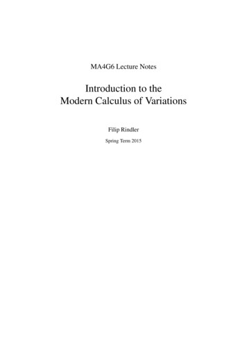
6CHAPTER 1. INTRODUCTIONleave out some of the rigorous detail that is expected in a graduate course. These firstfour chapters require some familiarity with ordinary differential equations (ODEs),and multi-variable calculus. The appendix contains some mathematical preliminariesand notational conventions that are important to review.The level of rigour increases dramatically in Chapter 4, where we begin a study ofthe direct method in the Calculus of Variations for proving existence of minimizers.This chapter requires some basic background in functional analysis and, in particular,Sobolev spaces. We provide a very brief overview in Section 4.2, and refer the readerto [28] for more details.Finally, in Chapter 5 we give an overview of applications of the calculus of variations to prove discrete to continuum results in graph-based semi-supervised learning.The ideas in this chapter are related to Γ-convergence, which is a notion of convergence for functionals that ensures minimizers converge to minimizers.These notes are just a basic introduction. We refer the reader to [28, Chapter8] and [22] for a more thorough exposition of the theory behind the Calculus ofVariations.1.1ExamplesWe begin with some examples.Example 1.1 (Shortest path). Let A and B be two points in the plane. Whatis the shortest path between A and B? The answer depends on how we measurelength! Suppose the length of a short line segment near (x, y) is the usual Euclideanlength multiplied by a positive scale factor g(x, y). For example, the length of a pathcould correspond to the length of time it would take a robot to navigate the path,and certain regions in space may be easier or harder to navigate, yielding larger orsmaller values of g. Robotic navigation is thus a special case of finding the shortestpath between two points.Suppose A lies to the left of B and the path is a graph u(x) over the x axis. SeeFigure 1.1. Then the “length” of the path between x and x x is approximatelypL g(x, u(x)) 1 u0 (x)2 x.If we let A (0, 0) and B (a, b) where a 0, then the length of a path (x, u(x))connecting A to B isZ apI(u) g(x, u(x)) 1 u0 (x)2 dx.0The problem of finding the shortest path from A to B is equivalent to finding thefunction u that minimizes the functional I(u) subject to u(0) 0 and u(a) b. 4
1.1. EXAMPLES7Figure 1.1: In our version of the shortest path problem, all paths must be graphs offunctions u u(x).Example 1.2 (Brachistochrone problem). In 1696 Johann Bernoulli posed the following problem. Let A and B be two points in the plane with A lying above B.Suppose we connect A and B with a thin wire and allow a bead to slide from A toB under the influence of gravity. Assuming the bead slides without friction, what isthe shape of the wire that minimizes the travel time of the bead? Perhaps counterintuitively, it turns out that the optimal shape is not a straight line! The problemis commonly referred to as the brachistochrone problem—the word brachistochronederives from ancient Greek meaning “shortest time”.Let g denote the acceleration due to gravity. Suppose that A (0, 0) and B (a, b) where a 0 and b 0. Let u(x) for 0 x a describe the shape of thewire, so u(0) 0 and u(a) b. Let v(x) denote the speed of the bead when it isat position x. When the bead is at position (x, u(x)) along the wire, the potentialenergy stored in the bead is PE mgu(x) (relative to height zero), and the kineticenergy is KE 21 mv(x)2 , where m is the mass of the bead. By conservation of energy1mv(x)2 mgu(x) 0,2since the bead starts with zero total energy at point A. Thereforepv(x) 2gu(x).Between x and x x,pthe bead slides a distance of approximatelywith a speed of v(x) 2gu(x). Hence it takes approximatelyp1 u0 (x)2t p x 2gu(x)p1 u0 (x)2 x
8CHAPTER 1. INTRODUCTIONFigure 1.2: Depiction of possible paths for the brachistochrone problem.time for the bead to move from position x to x x. Therefore the total time takenfor the bead to slide down the wire is given byZ as11 u0 (x)2I(u) dx. u(x)2g 0The problem of determining the optimal shape of the wire is therefore equivalent tofinding the function u(x) that minimizes I(u) subject to u(0) 0 and u(a) b. 4Example 1.3 (Minimal surfaces). Suppose we bend a piece of wire into a loop ofany shape we wish, and then dip the wire loop into a solution of soapy water. Asoap bubble will form across the loop, and we may naturally wonder what shape thebubble will take. Physics tells us that soap bubble formed will be the one with leastsurface area, at least locally, compared to all other surfaces that span the wire loop.Such a surface is called a minimal surface.To formulate this mathematically, suppose the loop of wire is the graph of afunction g : U R, where U R2 is open and bounded. We also assume that allpossible surfaces spanning the wire can be expressed as graphs of functions u : U R.To ensure the surface connects to the wire we ask that u g on U . The surfacearea of a candidate soap film surface u is given byZ pI(u) 1 u 2 dx.UThus, the minimal surface problem is equivalent to finding a function u that minimizesI subject to u g on U .4Example 1.4 (Image restoration). A grayscale image is a function u : [0, 1]2 [0, 1].For x R2 , u(x) represents the brightness of the pixel at location x. In real-world
1.1. EXAMPLES9applications, images are often corrupted in the acquisition process or thereafter, andwe observe a noisy version of the image. The task of image restoration is to recoverthe true noise-free image from a noisy observation.Let f (x) be the observed noisy image. A widely used and very successful approachto image restoration is the so-called total variation (TV) restoration, which minimizesthe functionalZ1(u f )2 λ u dx,I(u) U 2where λ 0 is a parameter and U (0, 1)2 . The restored image is the function uthat minimizes I (we do not impose boundary conditions on the minimizer). Thefirst term 12 (u f )2 is a called a fidelity term, and encourages the restored image tobe close to the observed noisy image f . The second term u measures the amountof noise in the image and minimizing this term encourages the removal ofR noise inthe restored image. The name TV restoration comes from the fact that U u dxis called the total variation of u. Total variation image restoration was pioneered byRudin, Osher, and Fatemi [49].4Example 1.5 (Image segmentation). A common task in computer vision is the segmentation of an image into meaningful regions. Let f : [0, 1]2 [0, 1] be a grayscaleimage we wish to segment. We represent possible segmentations of the image by thelevel sets of functions u : [0, 1]2 R. Each function u divides the domain [0, 1]2 intotwo regions defined byR (u) {x [0, 1]2 : u(x) 0} and R (u) {x [0, 1]2 : u(x) 0}.The boundary between the two regions is the level set {x [0, 1]2 : u(x) 0}.At a very basic level, we might assume our image is composed of two regions withdifferent intensity levels f a and f b, corrupted by noise. Thus, we might proposeto segment the image by minimizing the functionalZZ2I(u, a, b) (f (x) a) dx (f (x) b)2 dx,R (u)R (u)over all possible segmentations u and real numbers a and b. However, this turnsout not to work very well since it does not incorporate the geometry of the regionin any way. Intuitively, a semantically meaningful object in an image is usuallyconcentrated in some region of the image, and might have a rather smooth boundary.The minimizers of I could be very pathological and oscillate rapidly trying to captureevery pixel near a in one region and those near b in another region. For example, if fonly takes the values 0 and 1, then minimizing I will try to put all the pixels in theimage where f is 0 into one region, and all those where f is 1 into the other region,and will choose a 0 and b 1. This is true regardless of whether the region wheref is zero is a nice circle in the center of the image, or if we randomly choose each
10CHAPTER 1. INTRODUCTIONpixel to be 0 or 1. In the later case, the segmentation u will oscillate wildly and doesnot give a meaningful result.A common approach to fixing this issue is to include a penalty on the lengthof the boundary between the two regions. Let us denote the length of the boundarybetween R (u) and R (u) (i.e., the zero level set of u) by L(u). Thus, we seek insteadto minimize the functionalZZ2I(u, a, b) (f (x) a) dx (f (x) b)2 dx λL(u),R (u)R (u)where λ 0 is a parameter. Segmentation of an image is therefore reduced to findinga function u(x) and real numbers a and b minimizing I(u, a, b), which is a problemin the calculus of variations. This widely used approach was proposed by Chan andVese in 2001 and is called Active Contours Without Edges [20].The dependence of I on u is somewhat obscured in the form above. Let us writethe functional in another way. Recall the Heaviside function H is defined as(1, if x 0H(x) 0, if x 0.Then the region R (u) is precisely the region where H(u(x)) 1, and the regionR (u) is precisely where H(u(x)) 0. ThereforeZZ2(f (x) a) dx H(u(x))(f (x) a)2 dx,R (u)Uwhere U (0, 1)2 . LikewiseZZ2(1 H(u(x))) (f (x) b)2 dx.(f (x) b) dx R (u)UWe also have the identity (see Section A.10.2)ZZL(u) H(u(x)) dx δ(u(x)) u(x) dx.UUTherefore we haveZI(u, a, b) H(u)(f a)2 (1 H(u)) (f b)2 λδ(u) u dx.U4
Chapter 2The Euler-Lagrange equationWe aim to study general functionals of the formZL(x, u(x), u(x)) dx,(2.1)I(u) Uwhere U Rd is open and bounded, and L is a functionL : U R Rd R.The function L is called the Lagrangian. We will write L L(x, z, p) where x U ,z R and p Rd . Thus, z represents the variable where we substitute u(x), and p isthe variable where we substitute u(x). Writing this out completely we haveL L(x1 , x2 , . . . , xn , z, p1 , p2 , . . . , pn ).The partial derivatives of L will be denoted Lz (x, z, p), x L(x, z, p) (Lx1 (x, z, p), . . . , Lxn (x, z, p)),and p L(x, z, p) (Lp1 (x, z, p), . . . , Lpn (x, z, p)).Each example from Section 1.1 involved a functional of the general form of (2.1).For the shortest path problem d 1 andqL(x, z, p) g(x1 , z) 1 p21 .For the brachistochrone problem d 1 andsL(x, z, p) 111 p21. z
12CHAPTER 2. THE EULER-LAGRANGE EQUATIONFor the minimal surface problem n 2 andpL(x, z, p) 1 p 2 .For the image restoration problem n 2 and1L(x, z, p) (z f (x))2 λ p .2Finally, for the image segmentation problemL(x, z, p) H(z)(f (x) a)2 (1 H(z)) (f (x) b)2 λδ(z) p .We will always assume that L is smooth, and the boundary condition g : U Ris smooth. We now give necessary conditions for minimizers of I.Theorem 2.1 (Euler-Lagrange equation). Suppose that u C 2 (U ) satisfiesI(u) I(v)(2.2)for all v C 2 (U ) with v u on U . ThenLz (x, u, u) div ( p L(x, u, u)) 0(2.3)in U.Proof. Let ϕ Cc (U ) and set v u tϕ for a real number t. Since ϕ 0 on Uwe have u v on U . Thus, by assumptionI(u) I(v) I(u tϕ) for all t R.This means that h(t) : I(u tϕ) has a global minimum at t 0, i.e., h(0) h(t)for all t. It follows that h0 (t) 0, which is equivalent toddt(2.4)I(u tϕ) 0.t 0We now compute the derivative in (2.4). Notice thatZI(u tϕ) L(x, u(x) tϕ(x), u(x) t ϕ(x)) dx.UFor notational simplicity, let us suppress the x arguments from u(x) and ϕ(x). Bythe chain ruledL(x, u tϕ, u t ϕ) Lz (x, u tϕ, u t ϕ)ϕ p L(x, u tϕ, u t ϕ)· ϕ.dtThereforeddtt 0L(x, u tϕ, u t ϕ) Lz (x, u, u)ϕ p L(x, u, u) · ϕ,
13and we haveddt(2.5)ZdI(u tϕ) L(x, u(x) tϕ(x), u(x) t ϕ(x)) dxdt t 0 Ut 0Zd L(x, u(x) tϕ(x), u(x) t ϕ(x)) dxdt t 0UZLz (x, u, u)ϕ p L(x, u, u) · ϕ dx ZUZ Lz (x, u, u)ϕ dx p L(x, u, u) · ϕ dx.UUSince ϕ 0 on U we can use the Divergence Theorem (Theorem A.32) to computeZZ p L(x, u, u) · ϕ dx div ( p L(x, u, u)) ϕ dx.UUCombining this with (2.4) and (2.5) we haveZ d0 I(u tϕ) Lz (x, u, u) div ( p L(x, u, u)) ϕ dx.dt t 0UIt follows from the vanishing lemma (Lemma A.43 in the appendix) thatLz (x, u, u) div ( p L(x, u, u)) 0everywhere in U , which completes the proof.Remark 2.2. Theorem 2.1 says that minimizers of the functional I satisfy the PDE(2.3). The PDE (2.3) is called the Euler-Lagrange equation for I.Definition 2.3. A solution u of the Euler-Lagrange equation (2.3) is called a criticalpoint of I.Remark 2.4. In dimension d 1 we write x x1 and p p1 . Then the EulerLagrange equation isLz (x, u(x), u0 (x)) dLp (x, u(x), u0 (x)) 0.dxRemark 2.5. In the proof of Theorem 2.1 we showed thatZLz (x, u, u)ϕ p L(x, u, u) · ϕ dx 0Ufor all ϕ Cc (U ). A function u C 1 (U ) satisfying the above for all ϕ Cc (U ) iscalled a weak solution of the Euler-Lagrange equation (2.3). Thus, weak solutions ofPDEs arise naturally in the calculus of variations.
14CHAPTER 2. THE EULER-LAGRANGE EQUATIONExample 2.1. Consider the problem of minimizing the Dirichlet energyZ1 u 2 uf dx,(2.6)I(u) 2Uover all u satisfying u g on U . Here, f : U R and g : U R are givenfunctions, and1L(x, z, p) p 2 zf (x).2ThereforeLz (x, z, p) f (x) and p L(x, z, p) p,and the Euler-Lagrange equation is f (x) div( u) 0 in U.This is Poisson’s equation u f in Usubject to the boundary condition u g on U .4Exercise 2.6. Derive the Euler-Lagrange equation for the problem of minimizingZ1 u p uf dxI(u) pUsubject to u g on U , where p 1.4Example 2.2. The Euler-Lagrange equation in dimension d 1 can be simplifiedwhen L has no x-dependence, so L L(z, p). In this case the Euler-Lagrange equationreadsdLp (u(x), u0 (x)).Lz (u(x), u0 (x)) dxUsing the Euler-Lagrange equation and the chain rule we computedL(u(x), u0 (x)) Lz (u(x), u0 (x))u0 (x) Lp (u(x), u0 (x))u00 (x)dxd u0 (x) Lp (u(x), u0 (x)) Lp (u(x), u0 (x))u00 (x)dxd 0 (u (x)Lp (u(x), u0 (x))) .dxTherefored(L(u(x), u0 (x)) u0 (x)Lp (u(x), u0 (x))) 0.dxIt follows that(2.7)L(u(x), u0 (x)) u0 (x)Lp (u(x), u0 (x)) Cfor some constant C. This form of the Euler-Lagrange equation is often easier tosolve when L has no x-dependence.4
2.1. THE GRADIENT INTERPRETATION15In some of the examples presented in Section 1.1, such as the image segmentationand restoration problems, we did not impose any boundary condition on the minimizeru. For such problems, Theorem 2.1 still applies, but the Euler-Lagrange equation(2.3) is not uniquely solvable without a boundary condition. Hence, we need someadditional information about minimizers in order for the Euler-Lagrange equation tobe useful for these problems.Theorem 2.7. Suppose that u C 2 (U ) satisfiesI(u) I(v)(2.8)for all v C 2 (U ). Then u satisfies the Euler-Lagrange equation (2.3) with boundarycondition p L(x, u, u) · ν 0(2.9)on U.Proof. By Theorem 2.1, u satisfies the Euler-Lagrange equation (2.3). We just needto show that u also satisfies the boundary condition (2.9).Let ϕ C (U ) be a smooth function that is not necessarily zero on U . Thenby hypothesis I(u) I(u tϕ) for all t. Therefore, as in the proof of Theorem 2.1we haveZdLz (x, u, u)ϕ p L(x, u, u) · ϕ dx.(2.10)0 I(u tϕ) dt t 0UApplying the Divergence Theorem (Theorem A.32) we find thatZZ0 ϕ p L(x, u, u) · ν dS (Lz (x, u, u) div ( p L(x, u, u))) ϕ dx. UUSince u satisfies the Euler-Lagrange equation (2.3), the second term above vanishesand we haveZϕ p L(x, u, u) · ν dS 0 Ufor all test functions ϕ C (U ). By a slightly different version of the vanishinglemma (Lemma A.43 in the appendix) we have that p L(x, u, u) · ν 0 on U.This completes the proof.2.1The gradient interpretationWe can interpret the Euler-Lagrange equation (2.3) as the gradient of I. That is, ina certain sense (2.3) is equivalent to I(u) 0.
16CHAPTER 2. THE EULER-LAGRANGE EQUATIONTo see why, let us consider a function u : Rd R. The gradient of u is defined asthe vector of partial derivatives u(x) (ux1 (x), ux2 (x), . . . , uxn (x)).By the chain rule we haveddt(2.11)u(x tv) u(x) · vt 0for any vector v Rd . It is possible to take (2.11) as the definition of the gradient ofu. By this, we mean that w u(x) is the unique vector satisfyingddtu(x tv) w · vt 0for all v Rd .In the case of functionals I(u), we showed in the proof of Theorem 2.1 thatddtt 0I(u tϕ) (Lz (x, u, u) div ( p L(x, u, u)) , ϕ)L2 (U )for all ϕ Cc (U ). Here, the L2 -inner product plays the role of the dot product fromthe finite dimensional case. Thus, it makes sense to define the gradient, also calledthe functional gradient, to be(2.12) I(u) : Lz (x, u, u) div ( p L(x, u, u)) ,so that we have the identity(2.13)ddtt 0I(u tϕ) ( I(u), ϕ)L2 (U ) .The reader should compare this with the ordinary chain rule (2.11). Notice thedefinition of the gradient I depends on the choice of the L2 -inner product. Usingother inner products will result in different notions of gradient.2.2The Lagrange multiplierThere are many problems in the calculus of variations that involve constraints on thefeasible minimizers. A classic example is the isoperimetric problem, which correspondsto finding the shape of a simple closed curve that maximizes the enclosed area giventhe curve has a fixed length . Here we are maximizing the area enclosed by the curvesubject to the constraint that the length of the curve is equal to .Let J be a functional defined byZJ(u) H(x, u(x), u(x)) dx.U
2.2. THE LAGRANGE MULTIPLIER17We consider the problem of minimizing I(u) subject to the constraint J(u) 0. TheLagrange multiplier method gives necessary conditions that must be satisfied by anyminimizer.Theorem 2.8 (Lagrange multiplier). Suppose that u C 2 (U ) satisfies J(u) 0 andI(u) I(v)(2.14)for all v C 2 (U ) with v u on U and J(v) 0. Then there exists a real numberλ such that I(u) λ J(u) 0(2.15)in U.Here, I and J are the functional gradients of I and J, respectively, defined by(2.12).Remark 2.9. The number λ in Theorem 2.8 is called a Lagrange multiplier.Proof. We will give a short sketch of the proof. Let ϕ Cc (U ). Then as in Theorem2.1ddtt 0I(u tϕ) ( I(u), ϕ)L2 (U )andddtt 0J(u tϕ) ( J(u), ϕ)L2 (U ) .Suppose that ( J(u), ϕ)L2 (U ) 0. Then, up to a small approximation error0 J(u) J(u tϕ)for small t. Since ϕ 0 on U , we also have u u tϕ on U . Thus by hypothesisI(u) I(u tϕ) for all small t.Therefore, t 7 I(u tϕ) has a minimum at t 0 and so( I(u), ϕ)L2 (U ) ddtI(u tϕ) 0.t 0Hence, we have shown that for all ϕ Cc (U )( J(u), ϕ)L2 (U ) 0 ( I(u), ϕ)L2 (U ) 0.This says that I(u) is orthogonal to everything that is orthogonal to J(u). Intuitively this must imply that I(u) and J(u) are co-linear; we give the proofbelow.We now have three cases.1. If J(u) 0 then ( I(u), ϕ)L2 (U ) 0 for all ϕ C (U ), and by the vanishinglemma I(u) 0. Here we can choose any real number for λ.2. If I(u) 0 then we can take λ 0 to complete the proof.
18CHAPTER 2. THE EULER-LAGRANGE EQUATION3. Now we can assume I(u) 6 0 and J(u) 6 0. Defineλ ( I(u), J(u))L2 (U )k J(u)kL2 (U )and v I(u) λ J(u).By the definition of λ we can check that( J(u), v)L2 (U ) 0.Therefore ( I(u), v)L2 (U ) 0 and we have0 ( I(u), v)L2 (U ) (v λ J(u), v)L2 (U ) (v, v)L2 (U ) λ( J(u), v)L2 (U ) kvk2L2 (U ) .Therefore v 0 and so I(u) λ J(u) 0. This completes the proof.Remark 2.10. Notice that (2.15) is equivalent to the necessary conditions minimizersfor the augmented functionalK(u) I(u) λJ(u).2.3Gradient descentTo numerically compute solutions of the Euler-Lagrange equation I(u) 0, weoften use gradient descent, which corresponds to solving the PDE(2.16)(ut (x, t) I(u(x, t)), in U (0, )u(x, 0) u0 (x),on U {t 0}.We also impose the boundary condition u g or p L(x, u, u)·ν 0 on U (0, ),depending on which condition was imposed in the variational problem. Gradientdescent evolves u in the direction that decreases I most rapidly, starting at someinitial guess u0 . If we reach a stationary point where ut 0 then we have found asolution of the Euler-Lagrange equation I(u) 0. If solutions of the Euler-Lagrangeequation are not unique, we may find different solutions depending on the choice ofu0 .To see that gradient descent actually decreases I, let u(x, t) solve (2.16) and
2.3. GRADIENT DESCENT19computedI(u) dtZZUdL(x, u(x, t), u(x, t)) dxdtLz (x, u, u)ut p L(x, u, u) ut dx ZU(Lz (x, u, u) div ( p L(x, u, u))) ut dx U ( I(u), ut )L2 (U ) ( I(u), I(u))L2 (U ) k I(u)kL2 (U ) 0.We used integration by parts in the third line, mimicking the proof of Theorem 2.1.Notice that either boundary condition u g or p L(x, u, u) · ν 0 on U ensuresthe boundary terms vanish in the integration by parts.Notice that by writing out the Euler-Lagrange equation we can write the gradientdescent PDE (2.16) as(ut Lz (x, u, u) div ( p L(x, u, u)) 0, in U (0, )(2.17)u u0 , on U {t 0}.Example 2.3. Gradient descent on the Dirichlet energy (2.6) is the heat equation(ut u f, in U (0, )(2.18)u u0 , on U {t 0}.Thus, solving the heat equation is the fastest way to decrease the Dirichlet energy. 4We now prove that gradient descent converges to the unique solution of the EulerLagrange equation when I is strongly convex. For simplicity, we consider functionalsof the formZ(2.19)I(u) Ψ(x, u) Φ(x, u) dx.UThis includes the regularized variational problems used for image denoising in Example 1.4 and Section 3.6, for example. The reader may want to review definitions andproperties of convex functions in Section A.8 before reading the following theorem.Theorem 2.11. Assume I is given by (2.19), where z 7 Ψ(x, z) is θ-strongly convexfor θ 0 and p 7 Φ(x, p) is convex. Let u C 2 (U ) be any function satisfying(2.20) I(u ) 0in U.
20CHAPTER 2. THE EULER-LAGRANGE EQUATIONLet u(x, t) C 2 (U [0, )) be a solution of the gradient descent equation (2.16) andassume that u u on U for all t 0. Then(2.21)ku u k2L2 (U ) Ce 2θtfor all t 0,where C ku0 u k2L2 (U ) .Proof. Define the energy(2.22)11e(t) ku u k2L2 (U ) 22Z(u(x, t) u (x))2 dx.UWe differentiate e(t), use the equations solved by u and u and the divergence theoremto find thatZ0e (t) (u u )ut dxUZ ( I(u) I(u ))(u u ) dxZU (Ψz (x, u) Ψz (x, u ))(u u ) dxUZdiv( p Φ(x, u) p Φ(x, u ))(u u ) dx UZ (Ψz (x, u) Ψz (x, u ))(u u ) dxUZ ( p Φ(x, u) p Φ(x, u )) · ( u u ) dx.USince z 7 Ψ(x, z) is θ-strongly convex, Theorem A.38 yields(Ψz (x, u) Ψz (x, u ))(u u ) θ(u u )2 .Likewise, since p 7 Φ(x, p) is convex, Theorem A.38 implies that( p Φ(x, u) p Φ(x, u )) · ( u u ) 0.Therefore(2.23)0Ze (t) θ(u u )2 dx 2θe(t).UNoting thatd(e(t)e 2θt ) e0 (t)e 2θt 2θe(t)e 2θt 0,dt 2θtwe have e(t) e(0)e, which completes the proof.
2.4. ACCELERATED GRADIENT DESCENT21Remark 2.12. Notice that the proof of Theorem 2.11 shows that solutions of I(u) 0, subject to Dirichlet boundary condition u g on U , are unique.Remark 2.13. From an optimization or numerical analysis point of view, the exponential convergence rate (2.21) is a linear
The calculus of variations is a field of mathematics concerned with minimizing (or maximizing) functionals (that is, real-valued functions whose inputs are functions). The calculus of variations has a wide range of applications in physics, engineering, applied and pure mathematics, and is intimately connected to partial differential equations .