Transcription
The Calculus of VariationsM. Bendersky Revised, December 29, 2008 These notes are partly based on a course given by Jesse Douglas.1
Contents1 Introduction. Typical Problems52 Some Preliminary Results. Lemmas of the Calculus of Variations103 A First Necessary Condition for a Weak Relative Minimum: The Euler-LagrangeDifferential Equation154 Some Consequences of the Euler-Lagrange Equation. The Weierstrass-ErdmannCorner Conditions.205 Some Examples256 Extension of the Euler-Lagrange Equation to a Vector Function, Y(x)327 Euler’s Condition for Problems in Parametric Form (Euler-Weierstrass Theory) 368 Some More Examples449 The first variation of an integral, I(t) J[y(x, t)] R x2 (t) y(x,t)x1 (t) f (x, y(x, t), x )dx; Application to transversality.5410 Fields of Extremals and Hilbert’s Invariant Integral.5911 The Necessary Conditions of Weierstrass and Legendre.6312 Conjugate Points,Focal Points, Envelope Theorems6913 Jacobi’s Necessary Condition for a Weak (or Strong) Minimum: GeometricDerivation7514 Review of Necessary Conditions, Preview of Sufficient Conditions.7815 More on Conjugate Points on Smooth Extremals.8216 The Imbedding Lemma.872
17 The Fundamental Sufficiency Lemma.9118 Sufficient Conditions.9319 Some more examples.9620 The Second Variation. Other Proof of Legendre’s Condition.10021 Jacobi’s Differential Equation.10322 One Fixed, One Variable End Point.11323 Both End Points Variable11924 Some Examples of Variational Problems with Variable End Points12225 Multiple Integrals12626 Functionals Involving Higher Derivatives13227 Variational Problems with Constraints.13828 Functionals of Vector Functions: Fields, Hilbert Integral, Transversality inHigher Dimensions.15529 The Weierstrass and Legendre Conditions for n 2 Sufficient Conditions.16930 The Euler-Lagrange Equations in Canonical Form.17331 Hamilton-Jacobi Theory17731.1 Field Integrals and the Hamilton-Jacobi Equation. . . . . . . . . . . . . . . . . . . . 17731.2 Characteristic Curves and First Integrals . . . . . . . . . . . . . . . . . . . . . . . . . 18231.3 A theorem of Jacobi. . . . . . . . . . . . . . . . . . . . . . . . . . . . . . . . . . . . . 18731.4 The Poisson Bracket. . . . . . . . . . . . . . . . . . . . . . . . . . . . . . . . . . . . 18931.5 Examples of the use of Theorem (31.10) . . . . . . . . . . . . . . . . . . . . . . . . . 19032 Variational Principles of Mechanics.3192
33 Further Topics:1954
1Introduction. Typical ProblemsThe Calculus of Variations is concerned with solving Extremal Problems for a Functional. That is to say Maximum and Minimum problems for functions whose domain contains functions, Y (x) (or Y (x1 , · · · x2 ), or n-tuples of functions). The range of the functionalwill be the real numbers, RExamples:I. Given two points P1 (x1 , y1 ), P2 (x2 , y2 ) in the plane, joined by a curve, y f (x).Rx pThe Length Functional is given by L1,2 (y) x12 1 (y 0 )2 dx. The domain is the set of all {z}dscurves, y(x) C 1 such that y(xi ) yi , i 1, 2. The minimum problem for L[y] is solved bythe straight line segment P1 P2 .II. (Generalizing I) The problem of Geodesics, (or the shortest curve between two givenpoints) on a given surface. e.g. on the 2-sphere they are the shorter arcs of great circles(On the Ellipsoid Jacobi (1837) found geodesics using elliptical coördinates in terms ofHyperelliptic integrals, i.e.Zpf ( a0 a1 x · · · a5 x5 dx, f rational )a.III. In the plane, given points, P1 , P2 find a curve of given length ( P1 P2 ) which togetherRx pwith segment P1 P2 bounds a maximum area. In other words, given x12 1 (y 0 )2 dx,maximizeR x2x1ydxThis is an example of a problem with given constraints (such problems are also called5
isoperimetric problems). Notice that the problem of geodesics from P1 to P2 on a givensurface, F (x, y, z) 0 can also be formulated as a variational problem with constraints:GivenF (x, y, z) 0Findy(x), z(x) to minimizeR x2 qx1dy 2dz 21 ( dx) ( dx) dx,where y(xi ) yi , z(xi ) zi for i 1, 2.IV. Given P1 , P2 in the plane, find a curve, y(x) from P1 to P2 such that the surface of revolutionobtained by revolving the curve about the x-axis has minimum surface area. In other wordsminimize 2πR P2P1yds with y(xi ) yi , i 1, 2. If P1 and P2 are not too far apart, relative tox2 x1 then the solution is a Catenary (the resulting surface is called a Catenoid).Figure 1: CatenoidOtherwise the solution is Goldschmidt’s discontinuous solution (discovered in 1831) obtained by revolving the curve which is the union of three lines: the vertical line from P1to the point (x1 , 0), the vertical line from P2 to (x2 , 0) and the segment of the x-axis from(x1 , 0) to (x2 , 0).6
Figure 2: Goldscmidt Discontinuous solutionThis example illustrates the importance of the role of the category of functions allowed.If we restrict to continuous curves then there is a solution only if the points are close.If the points are far apart there is a solution only if allow piecewise continuous curves (i.e.continuous except possibly for finitely many jump discontinuities. There are similar meaningsfor piecewise class C n .)The lesson is that the class of unknown functions must be precisely prescribed. If othercurves are admitted into “competition” the problem may change. For example the onlysolutions to minimizingZL[y] defb(1 (y 0 )2 )2 dx,y(a) y(b) 0.aare polygonal lines with y 0 1.V.The Brachistochrone problem. This is considered the oldest problem in the Calculus ofVariations. Proposed by Johann Bernoulli in 1696: Given a point 1 higher than a point 2in a vertical plane, determine a (smooth) curve from 1 2 along which a mass can slide7
along the curve in minimum time (ignoring friction) with the only external force acting onthe particle being gravity.Many physical principles may be formulated in terms of variational problems. Specificallythe least-action principle is an assertion about the nature of motion that provides an alternative approach to mechanics completely independent of Newton’s laws. Not only does theleast-action principle offer a means of formulating classical mechanics that is more flexibleand powerful than Newtonian mechanics, but also variations on the least-action principlehave proved useful in general relativity theory, quantum field theory, and particle physics.As a result, this principle lies at the core of much of contemporary theoretical physics.VI. Isoperimetric problem In the plane, find among all closed curves,C, of length theone(s) of greatest area (Dido’s problem) i.e. representing the curve by (x(t), y(t)): givenRpR ẋ2 ẏ 2 dt maximize A 12 (xẏ ẋy)dt (recall Green’s theorem).CCVII.Minimal Surfaces Given a simple, closed curve, C in R3 , find a surface, say of class C 2 ,bounded by C of smallest area (see figure 3).8
Figure 3:Assuming a surface represented by z f (x, y), passes through C we wish to minimizeZZ s z z1 ( )2 ( )2 dxdy x yRProving the existence of minimal surface is Plateau’s problem which was solved by JesseDouglas in 1931.9
2Some Preliminary Results. Lemmas of the Calculus of Variationse 1 , x2 ]Notation 1. Denote the category of piecewise continuous functions on [x1 , x2 ]. by C[xe 1 , x2 ]. IfLemma 2.1. (Fundamental or Lagrange’s Lemma) Let M (x) C[x0 for all η(x) such that η(x1 ) η(x2 ) 0,η(x) C n ,R x2x1M (x)η(x)dx 0 n on [x1 , x2 ] thenM (x) 0 at all points of continuity.Proof : . Assume the lemma is false, say M (x) 0, M continuous at x. Then there exista neighborhood, Nx (x1 , x2 ) such that M (x) p 0 for x Nx . Now take η0 (x) def 0,in [x1 , x2 ] outside Nx(x x1 )n 1 (x2 x)n 1 , in NxThen η0 C n on [x1 , x2 ] andZZx2M (x)η0 (x)dx x1Zx2x1For the case n takeη0 x2M (x)η0 (x)dx p(x x1 )n 1 (x2 x)n 1 dx 0x1 0,in [x1 , x2 ] outside Nx11 e x x2 e x1 x , in Nxq.e.d.e 1 , x2 ]. IfLemma 2.2. Let M (x) C[xC ,R x2x1M (x)η 0 (x)dx 0 for all η(x) such that η η(x1 ) η(x2 ) 0 then M (x) c on its set of continuity.10
Proof : (After Hilbert, 1899) Let a, a0 be two points of continuity of M . Then for b, b0 withx1 a b a0 b0 x2 we construct a C function1 η1 (x) satisfying 0,on [x1 , a] and [b0 , x2 ] p (a constant 0),on [b, a0 ] increasing on [a, b], decreasing on [a0 , b0 ]Step 1: Let ηb0 be as in lemma (2.1)ηb0 0,in [x1 , x2 ] outside [a, b]11 e x x2 e x1 x , in [a, b]Step 2: For some c such that b c a0 and x1 x c setη1 (x) R bapZxηb0 (t)dtηb0 (t)dtaSimilarly for c x x2 define η1 (x) bypη1 (x) R b0bb (t)dt0 ηZ0ab0xbηb0 (t)dtwhere bηb0 (x) is defined similar to ηb0 (t) with [a0 , b0 ] replacing [a, b].NowZx2x1ZM (x)η10 (x)dxb aZM (x)η10 (x)dxb0 a0M (x)η10 (x)dxwhere M (x) is continuous on [a, b], [a0 , b0 ]. By the mean value theorem there are α [a, b], α0 [a0 , b0 ] such that the integral equals M (α)1Rbaη10 (x)dx M (α0 )R b0a0η10 (x)dx p(M (α) If M were differentiable the lemma would be an immediate consequence of integration by parts.11
M (α0 )). By the hypothesis this is 0. Thus in any neighborhood of a and a0 there exist α, α0such that M (α) M (α0 ). It follows that M (a) M (a0 ).q.e.d. η1 in lemma (2.2) may be assumed to be in C n . One uses the C n function from lemma(2.1) in the proof instead of the C function. It is the fact that we imposed the endpoint condition on the test functions, η, thatallows non-zero constants for M . In particular simply integrating the bump functionfrom lemma (2.1) does not satisfy the condition. The lemma generalizes to:Lemma 2.3. If M (x) is a piecewise continuous function such thatZx2M (x)η (n) (x)dx 0x1for every function that has a piecewise continuous derivative of order n and satisfiesη (k) (xi ) 0, i 1, 2,k n then M (x) is a polynomial of degree n 1.(see [AK], page 197).Definition 2.4. The normed linear space Dn (a, b) consist of all continuous functions, y(x) nC̃ n [a, b]2 with bounded norm y n Σi 0max y (i) (x) .3x1 x x2If a functional, J : Dn (a, b) R is continuous we say J is continuous with respect to Dn .2i.e. have continuous derivatives to order n except perhaps at a finite number of points.3 y n is a norm because f is assumed to be continuous on [a, b].12
The first examples we will study are functionals of the formZbJ[y] f (x, y, y 0 )dsae.g. the arc length functional. It is easy to see that such functionals will be continuous withrespect to D1 but are not continuous as functionals from C R. In general functionalswhich depend on the n-th derivative are continuous with respect to Dn , but not with respectto Dk , k n.We assume we are given a function, f (x, y, z) say of class C 3 for x [x1 , x2 ], and for y insome interval (or region, G, containing the point y (y1 , y2 , · · · , yn )) and for all real z (orall real vectors, z (z1 , z2 , · · · , zn )).Consider functions, y(x) D1 [x1 , x2 ] such that y(x) G. Let M be the set of all suchy(x). For any such y M the integralZJ[y] defbf (x, y(x), y 0 (x))dxadefines a functional J : M R.Problem: To find relative or absolute extrema of J.Definition 2.5. Let y y0 (x), a x b be a curve in M.(a) A strong ² neighborhood of y0 is the set of all y M in an ² ball centered at y0 in C.(b) a weak ² neighborhood of y0 is an ² ball in D1 centered at y0 .4For example let y(x) 1nsin(nx). If1n4 ² 1, then y0 lies in a strong ² neighborhood of y0 0 but not in aweak ² neighborhood.13
A function y0 (x) M furnishes a weak relative minimum for J[y] if and only if J[y0 ] J[y] for all y in a weak ² neighborhood of y0 . It furnishes a strong relative minimum ifJ[y0 ] J[y] for all y in a strong ² neighborhood of y0 . If the inequalities are true forall y M we say the minimum is absolute. If is replaced by the minimum becomesimproper. There are similar notions for maxima instead of minima5 . In light of the commentsabove regarding continuity of a functional, we are interested in finding weak minima andmaxima.Example(A Problem with no minimum)Consider the problem to minimizeZ1py 2 (y 0 )2 dxJ[y] 0on D1 {y C 1 [0, 1], y(0) 0, y(1) 1} Observe that J[y] 1. Now consider the sequenceof functions in D1 , yk (x) xk . ThenZJ[yk ] 1xk 1 Zx2 k 2 dx1 00xk 1 (x k)dx 1 1.k 1So inf (J[y]) 1 but there is no function, y, with J[y] 1 since J[y] 1.65Obviously the problem of finding a maximum for a functional J[y] is the same as finding the minimum for J[y]6Notice that the family of functions {xk } is not closed, nor is it equicontinuous. In particular Ascoli’s theorem isnot violated.14
3A First Necessary Condition for a Weak Relative Minimum:The Euler-Lagrange Differential EquationWe derive Euler’s equation (1744) for a function y0 (x) furnishing a weak relative (improper)extremum forR x2x1f (x, y, y 0 )dx.Definition 3.1 (The variation of a Functional, Gâteaux derivative, or the Directional derivative). Let J[y] be defined on a Dn . Then the first variation of J at y Dn in the directionof η Dn (also called the Gâteaux derivative) in the direction of η at y is defined as J[y ²η] J[y] J[y ²η] δJ² 0² ²² 0 deflimAssume y0 (x) C̃ 1 furnishes such a minimum. Let η(x) C 1 such that η(xi ) 0, i 1, 2. Let B 0 be a bound for η , η 0 on [x1 , x2 ]. Let ²0 0 be given. Imbed y0 (x)in the family y² y0 (x) ²η(x). Then y² (x) C̃ 1 and if ² ²0 ( B1 ), y² is in the weakdef²0 -neighborhood of y0 (x).Now J[y² ] is a real valued function of ² with domain ( ²0 , ²0 ), hence the fact that y0furnishes a weak relative extremum implies 0J[y² ] ²² 0We may apply Leibnitz’s rule at points wherefy (x, y0 (x), y00 (x))η(x) fy0 (x, y0 (x), y00 (x))η 0 (x) is continuous :ddJ[y² ] d²d²Zx2x1f (x, y0 ²η, y00 ²η 0 )dx 15
Zx2x1fy (x, y0 ²η, y00 ²η 0 )η fy0 (x, y0 ²η, y00 ²η 0 )η 0 dxTherefore(2)Z x2 d J[y² ] fy (x, y0 , y00 )η fy0 (x, y0 , y00 )η 0 dx 0d²² 0x1We now use integration by parts, to continue.Zx2Zfy ηdx η(x)(x1x x2 Z fy dx) x1x1x2Z(x1Zx0x2fy dx)η (x)dx x1x1Z(xfy dx)η 0 (x)dxx1HenceZZx2δJ x[fy0 x1fy dx]η 0 (x)dx 0x1for any class C 1 function η such that η(xi ) 0, i 1, 2 and f (x, y0 (x), y00 (x))η(x) continuous.By lemma (2.2) we have proven the followingTheorem 3.2 (Euler-Lagrange, 1744). If y0 (x) provides an extremum for the functionalJ[y] R x2x1f (x, y, y 0 )dx then fy0 Rxx1y0 (x), y00 (x) are continuous on [x1 , x2 ].7 0y0may have jump discontinuities.fy dx c at all points of continuity. i.e. everywhere7That is to say y0 may be a broken extremal sometimes called adiscontinuous solution. Also in order to use Leibnitz’s law for differentiating under the integral sign we only neededf to be of class C 1 . In fact no assumption about fx was needed.16
Notice that the Gâteaux derivative can be formed without reference to any norm. Henceif it not zero it precludes y0 (x) being a local minimum with respect to any norm.Corollary 3.3. At any x where fy (x, y0 (x), y00 (x)) is continuous8 y0 satisfies the EulerLagrange differential equationd(fy0 ) fy 0dxProof : At points of continuity of fy (x, y0 (x), y00 (x)) we havefy 0 Rxx1fy dx c. Differentiating both sides proves the corollary.Solutions of the Euler-Lagrange equation are called extremals. It is important to notethat the derivativedf0dx yis not assumed to exist, but is a consequence of theorem (3.2).In fact if y00 (x) is continuous the Euler-Lagrange equation is a second order differential00equation9 even though y may not exist.Example 3.4. Consider the functional J[y] R1 1y 2 (2x y 0 )2 dx where y( 1) 0,1. The Euler-Lagrange equation is2y(2x y 0 )2 d[ 2y 2 (2x y 0 )]dxThe minimum of J[y] is zero and is achieved by the function 0,for 1 x 0y0 (x) x2 , for 0 x 1.00y00 is continuous, y0 satisfies the Euler-Lagrange equation yet y0 (0) does not exist.8Hence wherever y00 (x) is continuous.9In the simple case of a functional defined byR x2x1f (x, y, y 0 )dx.17y(1)
A condition guaranteeing that an extremal, y0 (x), is of class C 2 will be given in (4.4).A curve furnishing a weak relative extremum may not provide an extremum if the collection of allowable curves is enlarged. In particular if one finds an extremum to a variationalproblem among smooth curves it may be the case that it is not an extremum when compared to all piecewise-smooth curves. The following useful proposition shows that this cannothappen.Proposition 3.5. Suppose a smooth curve, y y0 (x) gives the functional J[y] an extremumin the class of all admissible smooth curves in some weak neighborhood of y0 (x). Then yprovides an extremum for J[y] in the class of all admissible piecewise-smooth curves in thesame neighborhood.Proof : We prove (3.5) for curves in R1 . The case of a curve in Rn follows by applyingthe following construction coordinate wise. Assume y0 is not an extremum among piecewisesmooth curves. We show that curves with 1 corner offer no competition (the case of k cornersis similar). Suppose ỹ has a corner at x c with ỹ(xi ) y0 (xi ) i 1, 2 and provides asmaller value for the functional than y0 (x) i.e.J[ỹ] J[y0 ] h,h 0in a weak ²-neighborhood of y0 . We show that there exist yb(x) C 1 in the weak ²neighborhood of y0 (x) with J[by ] J[ỹ] h2 . Then ŷ is a smooth curve with J[ŷ] J[y0 ]which is a contradiction. Let y z̃ be the curve z̃ of the curve z0 dy0dxdỹ.dxThen z̃ lies in a 2² neighborhood(in the sup norm). For a small δ 0 construct a curve, z from18
(c δ, z̃(c δ)) to (c δ, z̃(c δ)) in the strip of width 2² about z0 such thatZZc δc δzdx c δOutside [c δ, c δ] set z dỹ.dxz̃dx.c δNow define ŷ(x) ỹ(x1 ) Rxx1zdx (see figure 6). If δ issufficiently small ŷ lies in a weak ² neighborhood of y0 and J[ỹ] J[ŷ] f (x, ŷ, ŷ 0 ) dx 12 h.Figure 4: Construction of z.19R c δc δ f (x, ỹ.ỹ 0 )
4Some Consequences of theEuler-Lagrange Equation.TheWeierstrass-Erdmann Corner Conditions.Notice that the Euler-Lagrange equation does not involve fx . There is a useful formulationwhich does.e1 extremal ofTheorem 4.1. Let y0 (x) be a CZ0R x2x1f (x, y, y 0 )dx. Then y0 satisfiesxf y fy0 fx dx c.x1In particular at points of continuity of y00 we have(3)d(f y 0 fy0 ) fx 0dx Similar to the remark after (3.3) we are not assumingd(f y 0 fy0 )dxexist. The derivativeexist as a consequence of the theorem.00 If y0 exist in [x1 , x2 ] then (3) becomes a second order differential equation for y0 .00 If y0 exist then (3) is a consequence of Corollary 3.3 as can be seen by expanding (3).Proof : (of Theorem 4.1) With a a constant, introduce new coordinates (u, v) in the planeby u x ay, v y. Hence the extremal curve, C has a parametric representation in theplane with parameter xu x ay(x), v y(x).20
We have x u av, y v. If a is sufficiently small the first of these equations may besolved for x in terms of u.10 . So for a sufficiently small the extremal may be described in(v, u) coordinates as v y(x(u)) v(u). In other words if the new (u, v)-axes make asufficiently small angle with the (x, y)-axes then equation y y0 (x), x1 x x2 becomesv v0 (u), x1 ay1 u1 u u2 x2 ay2 and every curve v v(u) in a sufficiently smallneighborhood of v0 is the transform of a curve y(x) that lies in a weak neighborhood of y0 (x).The functional J[y(x)] R x2x1f (x, y, y 0 )dx becomes J[v(u)] R u2u1F (u, v(u), v̇(u))du where v̇v̇(u))(1 denotes differentiation with respect to u and F (u, v(u), v̇(u)) f (u av(u), v(u), 1 av̇(u)av̇(u)).11 Therefore the Euler-Lagrange equation applied to F (u, v0 , v̇0 ) becomesZx ayFv̇ Fv du cx1 ay1but Fv̇ af fy 0; Fv1 av̇ (afx fy )(1 av̇). Thereforefy 0af 1 av̇Zx ay(afx fy )(1 av̇)du cx1 ay1Substituting back to (x, y) coordinates, noting thatZ011 av̇ 1 ay 0 yieldsxaf (1 ay )fy0 afx fy dx c.x1Subtract the Euler-Lagrange equation (3.2) and dividing by a proves the theorem. q.e.d.10since11 dydx [x xdv· dududxay(x) u] 1 ay 0 (x) and y D1 implies y 0 bounded on [x1 , x2 ].21
Applications: Suppose f (x, y, y 0 ) is independent of y. Then the Euler-Lagrange equation reduces todf0dx y 0 or fy0 c. Suppose f (x, y, y 0 ) is independent of x. Then (3) reduces tof y 0 fy0 c.Returning to broken extremals, i.e. extremals y0 (x) of class C̃ 1 where y0 (x) has only a finitenumber of jump discontinuities in [x1 , x2 ]. As functions of xZxx1Zfy (x, y0 (x), y00 (x)dxxandx1fx (x, y0 (x), y00 (x))dxoccurring in (3.2) and (4.1) respectively are continuous in x. Therefore fy0 (x, y0 (x), y00 (x))and f y 0 fy0 are continuous on [x1 , x2 ]. In particular at a corner, c [x1 , x2 ] of y0 (x) thismeansTheorem 4.2 (Weierstrass-Erdmann Corner Conditions).12fy0 (c, y0 (c), y00 (c )) fy0 (c, y0 (c), y00 (c )) (f y 0 fy0 ) c (f y 0 fy0 ) c Thus if there is a corner at c then fy0 (c, y0 (c), z) as a function of z assumes the samevalue for two different values of z. As a consequence of the theorem of the mean there mustbe a solution to fy0 y0 (c, y0 (c), z) 0. Therefore we have:12There will be applications in later sections.22
Corollary 4.3. If fy0 y0 6 0 then an extremal must be smooth (i.e. cannot have corners).The problem of minimizing J[y] R x2x1f (x, y, y 0 )dx is non-singular if fy0 y0 is 0 or 0throughout a region. Otherwise it is singular. A point (x0 , y0 , y00 ) of an extremal y0 (x) ofR x2f (x, y, y 0 )dx is non-singular if fy0 y0 (x0 , y0 (x), y00 ) 6 0. We will show in (4.4) that anx1extremal must have a continuous second derivative near a non-singular point.Suppose a variational problem is singular in a region, i.e. fy0 y0 (x, y, y 0 ) 0 in some(x, y, y 0 ) region. Then fy0 N (x, y) and f M (x, y) N (x, y)y 0 . Hence the EulerLagrange equation becomes Nx My 0 for extremals. Note that J[y] R x2x1R x2x1f (x, y, y 0 )dx M dx N dy. There are two cases:1. My Nx in a region. Then J[y] is independent of path from P1 toP2 . Therefore theproblem with fixed end points has no relevance.2. My Nx only along a curve y y0 (x) (i.e. My 6 Nx identically) then y0 (x) isthe unique extremum for J[y], provided this curve contains P1 , P2 since it is the onlysolution of the Euler-Lagrange equation.Theorem 4.4 (Hilbert). If y y0 (x) is an extremal ofR x2x1f (x, y, y 0 )dx and (x0 , y0 , y00 ) isnon-singular (i.e. fy0 y0 (x0 , y0 (x), y00 ) 6 0) then in some neighborhood of x0 y0 (x) is of classC 2.Proof : Consider the implicit equation in x and zZxfy0 (x, y0 (x), z) x1fy (x, y0 (x), y00 (x))dx c 023
Where c is as in the (3.2). Its locus contains the point (x x0 , z y00 (x0 )). By hypothesisthe partial derivative with respect to z of the left hand side is not equal to 0 at this point.Hence by the implicit function theorem we can solve for z( y 0 ) in terms of x for x near x0and obtain y 0 of class C 1 near x0 . Hence y 00 exists and is continuous.q.e.d.Near a non-singular point, (x0 , y0 , y00 ) we can expand the Euler-Lagrange equation andsolve for y 00(4)y 00 fy fy 0 x y 0 fy 0 yfy 0 y 0Near a non-singular point the Euler-Lagrange equation becomes (4). If f is of class C 3then the right hand side of (4) is a C 1 function of y 0 . Hence we can apply the existenceand uniqueness theorem of differential equations to deduce that there is one and only oneclass-C 2 extremal satisfying given initial conditions, (x0 , y0 (x), y00 ).24
5Some ExamplesShortest Length[Problem I of §1]Zx2p1 (y 0 )2 dx.J[y] x1This is an example of a functional with integrand independent of y (see the first applicationin §4), i.e. the Euler-Lagrange equation reduces to fy0 c or y01 (y 0 )2 c. Therefore y 0 awhich is the equation of a straight line.Notice that any integrand of the form f (x, y, y 0 ) g(y 0 ) similarly leads to straight linesolutions.Minimal Surface of Revolution[Problem IV of §1]Zx2J[y] yp1 (y 0 )2 dxx1This is an example of a functional with integrand of the type discussed in the second application in §4. So we have the differential equation:f y 0 fy 0 ypy(y 0 )2 c1 (y 0 )2 p1 (y 0 )2oryp1 (y 0 )2Sodxdy c.y 2 c2 cSet y c cosh t. ThenZxx x0dxdy cdy25Ztt0sinh tdt ct b.sinh t
So the solution to the Euler-Lagrange equation associated to the minimal surface of revolution problem isy c cosh(x b)csatisfying yi c cosh(xi b), i 1, 2cThis is the graph of a catenary. It is possible to find a catenary connecting P1 (x1 , y1 )to P2 (x2 , y2 ) if y1 , y2 are not too small compared to x2 x1 (otherwise we obtain theGoldschmidt discontinuous solution). Note that fy0 y0 y3(1 (y 0 )2 ) 2. So corners are possibleonly if y 0 (see corollary 4.3).The following may help explain the Goldschmidt solution. Consider the problem ofminimizing the cost of a taxi ride from point P1 to point P2 in the x, y plane. Say the costof the ride given by the y-coordinate. In particular it is free to ride along the x axis. Thefunctional that minimizes the cost of the ride is exactly the same as the minimum surfaceof revolution functional. If x1 is reasonably close to x2 then the cab will take a path that isgiven by a catenary. However if the points are far apart in the x direction it seem reasonablethe the shortest path is given by driving directly to the x-axis, travel for free until you areare at x2 then drive up to P2 . This is the Goldschmidt solution.The Brachistochrone problem[Problem V of §1]For simplicity, we assume the original point coincides with the origin. Since the velocityof motion along the curve is given byv ds pdx 1 (y0)2dtdt26
we havep1 (y 0 )2dxvdt Using the formula for kinetic energy we know that1 2mv mgy.2Substituting into the formula for dt we obtainp1 (y 0 )2 dx.2gydt So the time it takes to travel along the curve, y, is given by the the functionalRx q0 )2J[y] x12 1 (ydx. J[y] does not involve x so we have to solve the first order differentialyequation (where we write the constant as 1 )2b(5)11f y 0 fy0 p 2by 1 (y 0 )2We also havefy 0 y 0 13y(1 (y 0 )2 ) 2.So for the brachistochrone problem a minimizing arc can have no corners i.e. it is of class C 2 .Equation (5) may be solved by separating the variables, but to quote [B62] “it is easier if weprofit by the experience of others” and introduce a new variable u defined by the equationy 0 tan27usin u 21 cos u
Then y b(1 cos u). Nowdxdx dy1 cos u ( )( b sin u) b(1 cos u).dudy dusin uTherefore we have a parametric solution of the Euler-Lagrange equation for the brachistochrone problem:x a b(u sin u)y b(1 cos u)for some constants a and b13 . This is the equation of a cycloid. Recall this is the locus of apoint fixed on the circumference of a circle of radius b as the circle rolls on the lower side ofthe x-axis. One may show that there is one and only one cycloid passing through P1 and P2 .An (approximate) quotation from Bliss:The fact that the curve of quickest descent must be a cycloid is the famous resultdiscovered by James and John Bernoulli in 1697. The cycloid has a number ofremarkable properties and was much studied in the 17th century. One interestingfact: If the final position of descent is at the lowest point on the cycloid, thenthe time of descent of a particle starting at rest is the same no matter what theposition of the starting point on the cycloid may be.That the cycloid should be the solution of the brachistochrone problem was regardedwith wonder and admiration by the Bernoulli brothers.13u is an angle of rotation, not time.28
The Bernoulli’s did not have the Euler-Lagrange equation (which was discovered about60 years later). Johann Bernoulli derived equation (5) by a very clever reduction of theproblem to Snell’s law in optics (which is derived in most calculus classes as a consequenceof Fermat’s principle that light travels a path of least time). Recall that if light travels froma point (x1 , y1 ) in a homogenous medium M1 to a point (x2 , y2 ) (x1 x2 ) in a homogeneousmedium M2 which is separated from M1 by the line y y0 . Suppose the respective lightvelocities in the two media are u1 and u2 . Then the point of intersection of the light withthe line y y0 is characterized bysin a1u1 sin a2u2(see the diagram below).(x2,y2)a2y y0a1(x1,y1)Figure 5: Snell’s lawWe now consider a single optically inhomogeneous medium M in which the light velocityis given by a function, u(y). If we take u(y) 2gy then the path light will travel is thesame as that taken by a particle that minimizes the travel time. We approximate M by asequence of parallel-faced homogeneous media, M1 , M2 , · · · with Mi having constant velocity29
given by u(yi ) for some yi in the i-th band. Now by Snell’s law we havesin φ2sin φ1 ···u1u3i.e.sin φi Cuiwhere C is a constant.Figure 6: An Approximation to the Light PathNow take a limit as the number of bands approaches infinity with the maximal widthapproaching zero. We havesin φ Cuwhere φ is as in figure 7, below.30
Figure 7:In particular y 0 (x) cot φ, so that1sin φ p1 (y 0 )2.So we have deduced that the light ray will follow a path that satisfies the differential equationuIf the velocity, u, is given by 1p1 (y 0 )2 C.2gy we obtain equation (5).31
6Extension of the Euler-Lagrange Equation to a Vector Function, Y(x)We extend the previous results to the case ofZx2J[Y ] f (x, Y, Y 0 )ds,Y (x) (y1 (x), · · · , yn (x)),x1Y 0 (y10 (x), · · · , yn0 (x))For the most part the generalizations are straight forward.Let M be continuous vector valued functions which have continuous derivatives on [x1 , x2 ]except, perhaps, at a finite number of points. A strong ²-neighborhood of Y0 (x) M is an 2 epsilon neighborhood. i.e.n1{Y (x) M Y (x) Y0 (x) [ Σ (yi (x) yi0 (x))2 ] 2 ²}i 1For a weak ²-neighborhood add the condition Y 0 (x) Y00 (x) ².The first variation of
The Calculus of Variations . x2 ¡x1 then the solution is a Catenary (the resulting surface is called a Catenoid). Figure 1: Catenoid Otherwise the solution is Goldschmidt’s discontinuous solution (discovered in 1831) ob-tained by revolving the curve whi