Transcription
Stat ComputDOI 10.1007/s11222-016-9671-0Statistical analysis of differential equations: introducingprobability measures on numerical solutionsPatrick R. Conrad1 · Mark Girolami1,2 · Simo Särkkä3 · Andrew Stuart4 ·Konstantinos Zygalakis5Received: 5 December 2015 / Accepted: 5 May 2016 The Author(s) 2016. This article is published with open access at Springerlink.comAbstract In this paper, we present a formal quantificationof uncertainty induced by numerical solutions of ordinaryand partial differential equation models. Numerical solutions of differential equations contain inherent uncertaintiesdue to the finite-dimensional approximation of an unknownand implicitly defined function. When statistically analysingmodels based on differential equations describing physical,or other naturally occurring, phenomena, it can be important to explicitly account for the uncertainty introduced bythe numerical method. Doing so enables objective determination of this source of uncertainty, relative to otheruncertainties, such as those caused by data contaminatedwith noise or model error induced by missing physical orinadequate descriptors. As ever larger scale mathematicalmodels are being used in the sciences, often sacrificing complete resolution of the differential equation on the gridsused, formally accounting for the uncertainty in the numerical method is becoming increasingly more important. Thispaper provides the formal means to incorporate this uncer-tainty in a statistical model and its subsequent analysis.We show that a wide variety of existing solvers can berandomised, inducing a probability measure over the solutions of such differential equations. These measures exhibitcontraction to a Dirac measure around the true unknown solution, where the rates of convergence are consistent with theunderlying deterministic numerical method. Furthermore,we employ the method of modified equations to demonstrateenhanced rates of convergence to stochastic perturbationsof the original deterministic problem. Ordinary differential equations and elliptic partial differential equations areused to illustrate the approach to quantify uncertainty inboth the statistical analysis of the forward and inverseproblems.Keywords Numerical analysis · Probabilistic numerics ·Inverse problems · Uncertainty quantificationMathematics Subject Classification 62F15 · 65N75 ·65L20Electronic supplementary material The online version of thisarticle (doi:10.1007/s11222-016-9671-0) contains supplementarymaterial, which is available to authorized users.1 IntroductionBPatrick R. Conradp.conrad@warwick.ac.uk1.1 Motivation1Department of Statistics, University of Warwick, Coventry,UK2Present Address: Alan Turing Institute, London, UK3Department of Electrical Engineering and Automation, AaltoUniversity, Espoo, Finland4Department of Mathematics, University of Warwick,Coventry, UK5School of Mathematics, University of Edinburgh, Edinburgh,ScotlandThe numerical analysis literature has developed a large rangeof efficient algorithms for solving ordinary and partial differential equations, which are typically designed to solvea single problem as efficiently as possible (Hairer et al.1993; Eriksson 1996). When classical numerical methodsare placed within statistical analysis, however, we argue thatsignificant difficulties can arise as a result of errors in thecomputed approximate solutions. While the distributions ofinterest commonly do converge asymptotically as the solver123
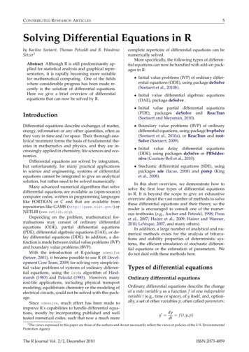
Stat Comput20151050 5 10 15 203020100 10 20 3050403020100the solver becomes completely inaccurate by the end of thedepicted interval given the step-size selected, the solver provides no obvious characterisation of its error at late times.Compare this with a sample of randomised solutions basedon the same integrator and the same step-size; it is obvious that early-time solutions are accurate and that theydiverge at late times, reflecting instability of the solver.Every curve drawn has the same theoretical accuracy asthe original classical method, but the randomised integrator provides a detailed and practical approach for revealingthe sensitivity of the solution to numerical errors. Themethod used requires only a straightforward modificationof the standard Runge–Kutta integrator and is explained inSect. 2.3.We summarise the contributions of this work as follows:– Construct randomised solvers of ODEs and PDEs usingnatural modification of popular, existing solvers.– Prove the convergence of the randomised methods andstudy their behaviour by showing a close link betweenrandomised ODE solvers and stochastic differentialequations (SDEs).– Demonstrate that these randomised solvers can be usedto perform statistical analyses that appropriately considersolver uncertainty.1.2 Review of existing workThe statistical analysis of models based on ordinary andpartial differential equations is growing in importance andzyFig. 1 A comparison ofsolutions to the Lorenz’63system using deterministic (red)and randomised (blue)integrators based on afourth-order Runge–Kuttaintegratorxmesh becomes dense [e.g. in statistical inverse problems(Dashti and Stuart 2016)], we argue that at a finite resolution, the statistical analyses may be vastly overconfident asa result of these unmodelled errors.The purpose of this paper is to address these issues bythe construction and rigorous analysis of novel probabilisticintegration methods for both ordinary and partial differentialequations. The approach in both cases is similar: we identify the key discretisation assumptions and introduce a localrandom field, in particular a Gaussian field, to reflect ouruncertainty in those assumptions. The probabilistic solvermay then be sampled repeatedly to interrogate the uncertainty in the solution. For a wide variety of commonly usednumerical methods, our construction is straightforward toapply and provably preserves the order of convergence of theoriginal method.Furthermore, we demonstrate the value of these probabilistic solvers in statistical inference settings. Analyticand numerical examples show that using a classical nonprobabilistic solver with inadequate discretisation whenperforming inference can lead to inappropriate and misleading posterior concentration in a Bayesian setting. In contrast,the probabilistic solver reveals the structure of uncertaintyin the solution, naturally limiting posterior concentration asappropriate.As a motivating example, consider the solution of theLorenz’63 system. Since the problem is chaotic, any typical fixed-step numerical methods will become increasinglyinaccurate for long integration times. Figure 1 depicts adeterministic solution for this problem, computed with afixed-step, fourth-order, Runge–Kutta integrator. Although1230510t1520
Stat Computa number of recent papers in the statistics literature havesought to address certain aspects specific to such models, e.g. parameter estimation (Liang and Wu 2008; Xueet al. 2010; Xun et al. 2013; Brunel et al. 2014) and surrogate construction (Chakraborty et al. 2013). However,the statistical implications of the reliance on a numerical approximation to the actual solution of the differentialequation have not been addressed in the statistics literature to date and this is the open problem comprehensivelyaddressed in this paper. Earlier work in the literature including randomisation in the approximate integration of ordinary differential equations (ODEs) includes (Coulibaly andLécot 1999; Stengle 1995). Our strategy fits within theemerging field known as Probabilistic Numerics (Henniget al. 2015), a perspective on computational methods pioneered by Diaconis (1988), and subsequently (Skilling 1992).This framework recasts solving differential equations as astatistical inference problem, yielding a probability measure over functions that satisfy the constraints imposed bythe specific differential equation. This measure formallyquantifies the uncertainty in candidate solution(s) of thedifferential equation, allowing its use in uncertainty quantification (Sullivan 2016) or Bayesian inverse problems(Dashti and Stuart 2016).A recent Probabilistic Numerics methodology for ODEs(Chkrebtii et al. 2013) [explored in parallel in Hennig andHauberg (2014)] has two important shortcomings. First, itis impractical, only supporting first-order accurate schemeswith a rapidly growing computational cost caused by thegrowing difference stencil [although Schober et al. (2014)extends to Runge–Kutta methods]. Secondly, this methoddoes not clearly articulate the relationship between theirprobabilistic structure and the problem being solved. Thesemethods construct a Gaussian process whose mean coincides with an existing deterministic integrator. While theyclaim that the posterior variance is useful, by the conjugacy inherent in linear Gaussian models, it is actuallyjust an a priori estimate of the rate of convergence ofthe integrator, independent of the actual forcing or initial condition of the problem being solved. These worksalso describe a procedure for randomising the construction of the mean process, which bears similarity to ourapproach, but it is not formally studied. In contrast, weformally link each draw from our measure to the analyticsolution.Our motivation for enhancing inference problems withmodels of discretisation error is similar to the more general concept of model error, as developed by Kennedy andO’Hagan (2001). Although more general types of modelerror, including uncertainty in the underlying physics, areimportant in many applications, our focus on errors arising from the discretisation of differential equations leads tomore specialised methods. Future work may be able to trans-late insights from our study of the restricted problem to themore general case. Existing strategies for discretisation errorinclude empirically fitted Gaussian models for PDE errors(Kaipio and Somersalo 2007) and randomly perturbed ODEs(Arnold et al. 2013); the latter partially coincides with ourconstruction, but our motivation and analysis are distinct.Recent work (Capistrán et al. 2013) uses Bayes factors toanalyse the impact of discretisation error on posterior approximation quality. Probabilistic models have also been used tostudy error propagation due to rounding error; see Haireret al. (2008).1.3 OrganisationThe remainder of the paper has the following structure:Sect. 2 introduces and formally analyses the proposed probabilistic solvers for ODEs. Section 3 explores the characteristics of random solvers employed in the statistical analysis ofboth forward and inverse problems. Then, we turn to ellipticPDEs in Sect. 4, where several key steps of the constructionof probabilistic solvers and their analysis have intuitive analogues in the ODE context. Finally, an illustrative exampleof an elliptic PDE inference problem is presented in Sect. 5.12 Probability measures via probabilistic timeintegratorsConsider the following ordinary differential equation (ODE):du f (u), u(0) u 0 ,dt(1)where u(·) is a continuous function taking values in Rn .2We let Φ t denote the flow map for Eq. (1), so that u(t) Φt u(0) . The conditions ensuring that this solution existswill be formalised in Assumption 2, below.Deterministic numerical methods for the integration ofthis equation on time interval [0, T ] will produce an approxK ,imation to the equation on a mesh of points {tk kh}k 0with K h T , (for simplicity we assume a fixed mesh). Letu k u(tk ) denote the exact solution of (1) on the mesh andUk u k denote the approximation computed using finiteevaluations of f . Typically, these methods output a singleK , often augmented with some typediscrete solution {Uk }k 0of error indicator, but do not statistically quantify the uncertainty remaining in the path.1Supplementary materials and code are available online: http://www2.warwick.ac.uk/pints.2To simplify our discussion we assume that the ODE is autonomous,that is, f (u) is independent of time. Analogous theory can be developedfor time-dependent forcing.123
Stat ComputLet X a,b denote the Banach space C([a, b]; Rn ). Theexact solution of (1) on the time interval [0, T ] may be viewedas a Dirac measure δu on X 0,T at the element u that solves theODE. We will construct a probability measure μh on X 0,T ,that is straightforward to sample from both on and off themesh, for which h quantifies the size of the discretisationstep employed, and whose distribution reflects the uncertainty resulting from the solution of the ODE. Convergenceof the numerical method is then related to the contraction ofμh to δu .We briefly summarise the construction of the numericalmethod. Let Ψh : Rn Rn denote a classical deterministic one-step numerical integrator over time-step h, a classincluding all Runge–Kutta methods and Taylor methods forODE numerical integration (Hairer et al. 1993). Our numerical methods will have the property that, on the mesh, theytake the formUk 1 Ψh (Uk ) ξk (h),(2)where ξk (h) are suitably scaled, i.i.d. Gaussian random variables. That is, the random solution iteratively takes thestandard step, Ψh , followed by perturbation with a randomdraw, ξk (h), modelling uncertainty that accumulates betweenK is straightforward tomesh points. The discrete path {Uk }k 0sample and in general is not a Gaussian process. Furthermore,the discrete trajectory can be extended into a continuous timeapproximation of the ODE, which we define as a draw fromthe measure μh .The remainder of this section develops these solvers indetail and proves strong convergence of the random solutions to the exact solution, implying that μh δu in anappropriate sense. Finally, we establish a close relationshipbetween our random solver and a stochastic differential equation (SDE) with small mesh-dependent noise. Intuitively,adding Gaussian noise to an ODE suggests a link to SDEs.Additionally, note that the mesh-restricted version of ouralgorithm, given by (2), has the same structure as a first-orderIto–Taylor expansion of the SDEdu f (u)dt σ dW,(3)for some choice of σ . We make this link precise by performing a backwards error analysis, which connects the behaviourof our solver to an associated SDE.2.1 Probabilistic time integrators: general formulationThe integral form of Eq. (1) is u(t) u 0 0123t f u(s) ds.(4)The solutions on the mesh satisfy tk 1u k 1 u k f u(s) ds,(5)tkand may be interpolated between mesh points by means ofthe expression u(t) u k t f u(s) ds, t [tk , tk 1 ).(6)tkWe may then write u(t) u k tg(s)ds, t [tk , tk 1 ),(7)tk where g(s) f u(s) is an unknown function of time. In thealgorithmic setting, we have approximate knowledge aboutg(s) through an underlying numerical method. A variety oftraditional numerical algorithms may be derived based onapproximation of g(s) by various simple deterministic functions g h (s). The simplest such numerical method arises frominvoking the Euler approximation thatg h (s) f (Uk ), s [tk , tk 1 ).(8)In particular, if we take t tk 1 and apply this method inductively the corresponding numerical scheme arising frommaking such an approximation to g(s) in (7) is Uk 1 Uk h f (Uk ). Now consider the more general one-stepnumerical method Uk 1 Ψh (Uk ). This may be derivedby approximating g(s) in (7) byg h (s) d Ψτ (Uk ), s [tk , tk 1 ).τ s tkdτ(9)We note that all consistent (in the sense of numerical analysis)one-step methods will satisfy d Ψτ (u) f (u).τ 0dτThe approach based on the approximation (9) leads to adeterministic numerical method which is defined as a continuous function of time. Specifically, we have U (s) Ψs tk (Uk ), s [tk , tk 1 ). Consider again the Euler approximation, for which Ψτ (U ) U τ f (U ), and whosecontinuous time interpolant is then given by U (s) Uk (s tk ) f (Uk ), s [tk , tk 1 ). Note that this producesa continuous function, namely an element of X 0,T , whenextended to s [0, T ]. The preceding development of anumerical integrator does not acknowledge the uncertaintythat arises from lack of knowledge about g(s) in the interval
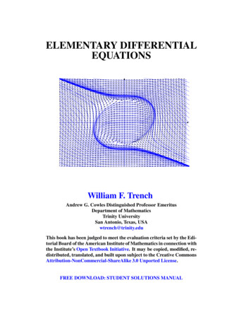
Stat Computs [tk , tk 1 ). We propose to approximate g stochasticallyin order to represent this uncertainty, takingg h (s) d Ψτ (Uk ) χk (s tk ), s [tk , tk 1 )τ s tkdτwhere the {χk } form an i.i.d. sequence of Gaussian randomfunctions defined on [0, h] with χk N (0, C h ).3We will choose C h to shrink to zero with h at a prescribedrate (see Assumption 1), and also to ensure that χk X 0,halmost surely. The functions {χk } represent our uncertaintyabout the function g. The corresponding numerical schemearising from such an approximation is given byUk 1 Ψh (Uk ) ξk (h),(a)(10)where the i.i.d. sequence of functions {ξk } lies in X 0,h and isgiven by ξk (t) tχk (τ )dτ.(11)0(b)Note that the numerical solution is now naturally definedbetween grid points, via the expressionU (s) Ψs tk (Uk ) ξk (s tk ), s [tk , tk 1 ).(12)When it is necessary to evaluate a solution at multiple pointsin an interval, s (tk , tk 1 ], the perturbations ξk (s tk )must be drawn jointly, which is facilitated by their Gaussianstructure. Although most users will only need the formulationon mesh points, we must consider off-mesh behaviour torigorously analyse higher order methods, as is also requiredfor the deterministic variants of these methods.In the case of the Euler method, for example, we haveUk 1 Uk h f (Uk ) ξk (h)(13)and, between grid points,While we argue that the choice of modelling local uncertainty in the flow map as a Gaussian process is naturaland analytically favourable, it is not unique. It is possible to construct examples where the Gaussian assumptionis invalid; for example, when a highly inadequate timestep is used, a systemic bias may be introduced. However,in regimes where the underlying deterministic method performs well, the centred Gaussian assumption is a reasonableprior.2.2 Strong convergence resultU (s) Uk (s tk ) f (Uk ) ξk (s tk ), s [tk , tk 1 ).(14)This method is illustrated in Fig. 2. Observe that Eq. (13)has the same form as an Euler–Maryama method for anassociated SDE (3) where σ depends on the step-size h. Inparticular, in the simple one-dimensional case, σ would begiven by C h / h. Section 2.4 develops a more sophisticatedconnection that extends to higher order methods and off themesh.We use χk N (0, C h ) to denote a zero-mean Gaussian processdefined on [0, h] with a covariance kernel cov(χk (t), χk (s)) C h (t, s).3Fig. 2 An illustration of deterministic Euler steps and randomised variations. The random integrator in (b) outputs the path in red; we overlaythe standard Euler step constructed at each step, before it is perturbed(blue)To prove the strong convergence of our probabilistic numerical solver, we first need two assumptions quantifying properties of the random noise and of the underlying deterministicintegrator, respectively. In what follows we use ·, · and · to denote the Euclidean inner product and norm on Rn . Wedenote the Frobenius norm on Rn n by · F , and Eh denotesexpectation with respect to the i.i.d. sequence {χk }. tAssumption 1 Let ξk (t) : 0 χk (s)ds with χk N (0, C h ).Then there exists K 0, p 1 such that, for all t [0, h],Eh ξk (t)ξk (t)T 2F K t 2 p 1 ; in particular Eh ξk (t) 2 K t 2 p 1 . Furthermore, we assume the existence of matrixQ, independent of h, such that Eh [ξk (h)ξk (h)T ] Qh 2 p 1 .123
Stat ComputHere, and in the sequel, K is a constant independent of h,but possibly changing from line to line. Note that the covariance kernel C h is constrained, but not uniquely defined. Wewill assume the form of the constant matrix is Q σ I , andwe discuss one possible strategy for choosing σ in Sect. 3.1.Section 2.4 uses a weak convergence analysis to argue thatonce Q is selected, the exact choice of C h has little practicalimpact.Assumption 2 The function f and a sufficient number of itsderivatives are bounded uniformly in Rn in order to ensurethat f is globally Lipschitz and that the numerical flow mapΨh has uniform local truncation error of order q 1:sup Ψt (u) Φt (u) K t q 1 .u RnRemark 2.1 We assume globally Lipschitz f , and boundedderivatives, in order to highlight the key probabilistic ideas,whilst simplifying the numerical analysis. Future work willaddress the non-trivial issue of extending of analyses toweaken these assumptions. In this paper, we provide numerical results indicating that a weakening of the assumptions isindeed possible.Theorem 2.2 Under Assumptions 1, 2 it follows that thereis K 0 such thatsup Eh u k Uk 2 K h 2 min{ p,q} .0 kh TFurthermore,sup Eh u(t) U (t) K h min{ p,q} .0 t TThis theorem implies that every probabilistic solution is agood approximation of the exact solution in both a discreteand continuous sense. Choosing p q is natural if we wantto preserve the strong order of accuracy of the underlyingdeterministic integrator; we proceed with the choice p q,introducing the maximum amount of noise consistent withthis constraint.2.3 Examples of probabilistic time integratorsThe canonical illustration of a probabilistic time integrator isthe probabilistic Euler method already described.4 Anotheruseful example is the classical Runge–Kutta method whichdefines a one-step numerical integrator as follows:Ψh (u) u h k1 (u) 2k2 (u, h) 2k3 (u, h) k4 (u, h) ,6where 1k1 (u) f (u), k2 (u, h) f u hk1 (u)2 1k3 (u, h) f u hk2 (u) , k4 (u, h) f u hk3 (u) .2The method has local truncation error in the form of Assumption 2 with q 4. It may be used as the basis of a probabilisticnumerical method (12), and hence (10) at the grid points.Thus, provided that we choose to perturb this integrator witha random process χk satisfying Assumption 1 with p 4,5Theorem 2.2 shows that the error between the probabilisticintegrator based on the classical Runge–Kutta method is, inthe mean square sense, of the same order of accuracy as thedeterministic classical Runge–Kutta integrator.2.4 Backward error analysisBackwards error analyses are useful tool for numerical analysis; the idea is to characterise the method by identifying amodified equation (dependent upon h) which is solved bythe numerical method either exactly, or at least to a higherdegree of accuracy than the numerical method solves theoriginal equation. For our random ODE solvers, we will showthat the modified equation is a stochastic differential equation(SDE) in which only the matrix Q from Assumption 1 enters;the details of the random processes used in our constructiondo not enter the modified equation. This universality property underpins the methodology we introduce as it shows thatmany different choices of random processes all lead to thesame effective behaviour of the numerical method.We introduce the operators L and Lh defined so that, forall φ C (Rn , R), h φ Φh (u) eh L φ (u), Eφ U1 U0 u eh L φ (u).(15)Thus L : f · and eh L is the kernel for the Markovchain generated by the probabilistic integrator (2). In fact wenever need to work with Lh itself in what follows, only withheh L , so that questions involving the operator logarithm donot need to be discussed.We now introduce a modified ODE and a modified SDEwhich will be needed in the analysis that follows. The modified ODE ishdû f h (û)dt(16)4An additional example of a probabilistic integrator, based on aOrnstein–Uhlenbeck process, is available in the supplementary materials.1235Implementing Eq. 10 is trivial, since it simply adds an appropriatelyscaled Gaussian random number after each classical Runge–Kutta step.
Stat Computwhilst the modified SDE has the form dũ f h (ũ)dt h 2 p Q dW.Finally we note that (20) implies that(17)The precise choice of f h is detailed below. Letting E denoteexpectation with respect to W , we introduce the operators Lhand Lh so that, for all φ C (Rn , R), h φ û(h) û(0) u eh L φ (u),(18) h Lh Eφ ũ(h) ũ(0) 0 e φ (u).(19)Thus,hh O(h 4 p 2 ) .Thus we have1L : f · , L f · h 2 p Q : ,2heh L φ(u) eh L φ(u) h 1 2 p 1 Q: I φ(u) eh L e 2 h h 1 2 p 1hQ : φ(u) O(h 4 p 2 ) eh L2 1 2 p 1hQ : φ(u) I O(h) 2hhh(20)where : denotes the inner product on Rn n which induces theFrobenius norm, that is, A:B trace(A T B).The fact that the deterministic numerical integrator hasuniform local truncation error of order q 1 (Assumption 2)implies that, since φ C ,eh L φ(u) φ(Ψh (u)) O(h q 1 ).(21)The theory of modified equations for classical one-stepnumerical integration schemes for ODEs (Hairer et al. 1993)establishes that it is possible to find f h in the formq lf h : f h i fi ,(22)eh L φ(u) φ(Ψh (u)) O(h q 2 l ).(23)i qsuch thathWe work with this choice of f h in what follows.Now for our stochastic numerical method we haveφ(Uk 1 ) φ(Ψh (Uk )) ξk (h) · φ(Ψh (Uk ))1 ξk (h)ξkT (h) : φ(Ψh (Uk )) O( ξk (h) 3 ).24 ).Furthermore, the last term has mean of size O( ξk (h) TFrom Assumption 1 we know that Eh ξk (h)ξk (h) Qh 2 p 1 . Thus heh L φ(u) φ Ψh (u) 1 h 2 p 1 Q : φ Ψh (u) O(h 4 p 2 ).(24)2From this it follows that heh L φ(u) φ Ψh (u)1 h 2 p 1 Q : φ(u) O(h 2 p 2 ).2(25)eh L φ(u) eh L φ(u) hh1 2 p 1Q : φ(u) O(h 2 p 2 ).h2(26)Now using (23), (25), and (26) we obtaineh L φ(u) eh L φ(u) O(h 2 p 2 ) O(h q 2 l ).hh(27)Balancing these terms, in what follows we make the choicel 2 p q. If l 0 we adopt the convention that the driftf h is simply f. With this choice of q we obtaineh L φ(u) eh L φ(u) O(h 2 p 2 ).hh(28)This demonstrates that the error between the Markov kernel of one-step of the SDE (17) and the Markov kernel of thenumerical method (2) is of order O(h 2 p 2 ). Some straightforward stability considerations show that the weak error overan O(1) time interval is O(h 2 p 1 ). We make assumptionsgiving this stability and then state a theorem comparing theweak error with respect to the modified Eq. (17), and theoriginal Eq. (1).Assumption 3 The function f is in C and all its derivatives are uniformly bounded on Rn . Furthermore, f ishsuch that the operators eh L and eh L satisfy, for all ψ C (Rn , R) and some L 0,sup eh L ψ(u) (1 Lh) sup ψ(u) ,u Rnsup eu Rnu Rnh Lhψ(u) (1 Lh) sup ψ(u) .u RnRemark 2.3 If p q in what follows (our recommendedchoice) then the weak order of the method coincides withthe strong order; however, measured relative to the modifiedequation, the weak order is then one plus twice the strongorder. In this case, the second part of Theorem 2.2 givesus the first weak order result in Theorem 2.4. Additionally,Assumption 3 is stronger than we need, but allows us tohighlight probabilistic ideas whilst keeping overly technical123
Stat Computaspects of the numerical analysis to a minimum. More sophisticated, but structurally similar, analysis would be requiredfor weaker assumptions on f . Similar considerations applyto the assumptions on φ.Theorem 2.4 Consider the numerical method (10) andassume that Assumptions 1 and 3 are satisfied. Then, forφ C function with all derivatives bounded uniformly onRn , we have that φ(u(T )) Eh φ(Uk ) K h min{2 p,q} , kh T,and E φ(ũ(T )) Eh φ(Uk ) K h 2 p 1 , kh T,where u and ũ solve (1) and (17), respectively.Example 2.5 Consider the probabilistic integrator derivedfrom the Euler method in dimension n 1. We thus haveq 1, and we hence set p 1. The results in Hairer et al.(2006) allow us to calculate f h with l 1. The precedingtheory then leads to strong order of convergence 1, measuredrelative to the true ODE (1), and weak order 3 relative to theSDEdû h2 hf (û) f (û) f (û) f 2 (û)212 4( f (û))2 f (û) dt ChdW.f (û) These results allow us to constrain the behaviour of therandomised method using limited information about thecovariance structure, C h . The randomised solution convergesweakly, at a high rate, to a solution that only depends on Q.Hence, we conclude that the practical behaviour of the solution is only dependent upon Q, and otherwise, C h may beany convenient kernel. With these results now available, thefollowing section provides an empirical study of our probabilistic integrators.3 Statistical inference and numericsThis section explores applications of the randomised ODEsolvers developed in Sect. 2 to forward and inverse problems. Throughout this section, we use the FitzHugh–Nagumomodel to illustrate ideas (Ramsay et al. 2007). This is a twostate non-linear oscillator, with states (V, R) and parameters(a, b, c), governed by the equationsV3dV c V R ,dt3123dR1 (V a b R) .dtc(29)This particular example does not satisfy the stringentAssumptions 2 and 3 and the numerical results shown demonstrate that, as indicated in Remarks 2.1 and 2.3, our theorywill extend to weaker assumptions on f , something we willaddress in future work.3.1 Calibrating forward uncertainty propagationConsider Eq. (29) with fixed initial conditions V (0) 1, R(0) 1, and parameter values (.2, .2, 3). Figure 3shows draws of the V species trajectories from the measureassociated with the probabilistic Euler solver with p q 1, for various values of the step-size and fixed σ 0.1.The random draws exhibit non-Gaussian structure at largestep-size and clearly contract towards the true solution.Although the rate of contraction is governed by theunderlying deterministic method, the scale parameter, σ ,completely controls the apparent uncertainty in the solver.6This tuning problem exists in general, since σ is problemdependent and cannot obviously be computed analytically.Therefore, we propose to calibrate σ to replicate theamount of error suggested by classical error indicators. In thefollowing discussion, we often explicitly denote the dependence on h and σ with superscripts, hence the probabilisticsolver is U h,σ and the corresponding deterministic solver isU h,0 . Define the deterministic erro
Lorenz'63 system. Since the problem is chaotic, any typi-cal fixed-step numerical methods will become increasingly inaccurate for long integration times. Figure 1 depicts a deterministic solution for this problem, computed with a fixed-step, fourth-order, Runge-Kutta integrator. Although the solver becomes completely inaccurate by the end .