Transcription
LECTURE SLIDES ON DYNAMIC PROGRAMMINGBASED ON LECTURES GIVEN AT THEMASSACHUSETTS INSTITUTE OF TECHNOLOGYCAMBRIDGE, MASSFALL 2004DIMITRI P. BERTSEKASThese lecture slides are based on the book:“Dynamic Programming and Optimal Control: 2nd edition,” Vols. I and II, AthenaScientific, 2002, by Dimitri P. st Updated: December 2004The slides are copyrighted, but may be freelyreproduced and distributed for any noncommercial purpose.
LECTURE CONTENTS These slides consist of 24 Lectures, whose summary is given in the next 24 slides Lectures 1-2: Basic dynamic programming algorithm (Chapter 1) Lectures 3-4: Deterministic discrete-time andshortest path problems (Chapter 2) Lectures 5-6: Stochastic discrete-time problems(Chapter 4) Lectures 7-9: Deterministic continuous-time optimal control (Chapter 4) Lectures 10-12: Problems of imperfect stateinformation (Chapter 5) Lectures 13-16: Approximate DP - suboptimalcontrol (Chapter 6) Lectures 17-20: Introduction to infinite horizonproblems (Chapter 7) Lectures 21-24: Advanced topics on infinitehorizon and approximate DP (Volume II)
6.231 DYNAMIC PROGRAMMINGLECTURE 1LECTURE OUTLINE Problem Formulation Examples The Basic Problem Significance of Feedback
6.231 DYNAMIC PROGRAMMINGLECTURE 2LECTURE OUTLINE The basic problem Principle of optimality DP example: Deterministic problem DP example: Stochastic problem The general DP algorithm State augmentation
6.231 DYNAMIC PROGRAMMINGLECTURE 3LECTURE OUTLINE Deterministic finite-state DP problems Backward shortest path algorithm Forward shortest path algorithm Shortest path examples Alternative shortest path algorithms
6.231 DYNAMIC PROGRAMMINGLECTURE 4LECTURE OUTLINE Label correcting methods for shortest paths Variants of label correcting methods Branch-and-bound as a shortest path algorithm
6.231 DYNAMIC PROGRAMMINGLECTURE 5LECTURE OUTLINE Examples of stochastic DP problems Linear-quadratic problems Inventory control
6.231 DYNAMIC PROGRAMMINGLECTURE 6LECTURE OUTLINE Stopping problems Scheduling problems Other applications
6.231 DYNAMIC PROGRAMMINGLECTURE 7LECTURE OUTLINE Deterministic continuous-time optimal control Examples Connection with the calculus of variations The Hamilton-Jacobi-Bellman equation as acontinuous-time limit of the DP algorithm The Hamilton-Jacobi-Bellman equation as asufficient condition Examples
6.231 DYNAMIC PROGRAMMINGLECTURE 8LECTURE OUTLINE Deterministic continuous-time optimal control From the HJB equation to the Pontryagin Minimum Principle Examples
6.231 DYNAMIC PROGRAMMINGLECTURE 9LECTURE OUTLINE Deterministic continuous-time optimal control Variants of the Pontryagin Minimum Principle Fixed terminal state Free terminal time Examples Discrete-Time Minimum Principle
6.231 DYNAMIC PROGRAMMINGLECTURE 10LECTURE OUTLINE Problems with imperfect state info Reduction to the perfect state info case Machine repair example
6.231 DYNAMIC PROGRAMMINGLECTURE 11LECTURE OUTLINE Review of DP for imperfect state info Linear quadratic problems Separation of estimation and control
6.231 DYNAMIC PROGRAMMINGLECTURE 12LECTURE OUTLINE DP for imperfect state info Sufficient statistics Conditional state distribution as a sufficientstatistic Finite-state systems Examples
6.231 DYNAMIC PROGRAMMINGLECTURE 13LECTURE OUTLINE Suboptimal control Certainty equivalent control Implementations and approximations Issues in adaptive control
6.231 DYNAMIC PROGRAMMINGLECTURE 14LECTURE OUTLINE Limited lookahead policies Performance bounds Computational aspects Problem approximation approach Vehicle routing example Heuristic cost-to-go approximation Computer chess
6.231 DYNAMIC PROGRAMMINGLECTURE 15LECTURE OUTLINE Rollout algorithms Cost improvement property Discrete deterministic problems Sequential consistency and greedy algorithms Sequential improvement
6.231 DYNAMIC PROGRAMMINGLECTURE 16LECTURE OUTLINE More on rollout algorithms Simulation-based methods Approximations of rollout algorithms Rolling horizon approximations Discretization issues Other suboptimal approaches
6.231 DYNAMIC PROGRAMMINGLECTURE 17LECTURE OUTLINE Infinite horizon problems Stochastic shortest path problems Bellman’s equation Dynamic programming – value iteration Examples
6.231 DYNAMIC PROGRAMMINGLECTURE 18LECTURE OUTLINE Stochastic shortest path problems Policy iteration Linear programming Discounted problems
6.231 DYNAMIC PROGRAMMINGLECTURE 19LECTURE OUTLINE Average cost per stage problems Connection with stochastic shortest path problems Bellman’s equation Value iteration Policy iteration
6.231 DYNAMIC PROGRAMMINGLECTURE 20LECTURE OUTLINE Control of continuous-time Markov chains –Semi-Markov problems Problem formulation – Equivalence to discretetime problems Discounted problems Average cost problems
6.231 DYNAMIC PROGRAMMINGLECTURE 21LECTURE OUTLINE With this lecture, we start a four-lecture sequence on advanced dynamic programming andneuro-dynamic programming topics. References: Dynamic Programming and Optimal Control, Vol. II, by D. Bertsekas Neuro-Dynamic Programming, by D. Bertsekas and J. Tsitsiklis 1st Lecture: Discounted problems with infinitestate space, stochastic shortest path problem 2nd Lecture: DP with cost function approximation 3rd Lecture: Simulation-based policy and valueiteration, temporal difference methods 4th Lecture: Other approximation methods:Q-learning, state aggregation, approximate linearprogramming, approximation in policy space
6.231 DYNAMIC PROGRAMMINGLECTURE 22LECTURE OUTLINE Approximate DP for large/intractable problems Approximate policy iteration Simulation-based policy iteration Actor-critic interpretation Learning how to play tetris: A case study Approximate value iteration with function approximation
6.231 DYNAMIC PROGRAMMINGLECTURE 23LECTURE OUTLINE Simulation-based policy and value iteration methods λ-Least Squares Policy Evaluation method Temporal differences implementation Policy evaluation by approximate value iteration TD(λ)
6.231 DYNAMIC PROGRAMMINGLECTURE 24LECTURE OUTLINE Additional methods for approximate DP Q-Learning Aggregation Linear programming with function approximation Gradient-based approximation in policy space
6.231 DYNAMIC PROGRAMMINGLECTURE 1LECTURE OUTLINE Problem Formulation Examples The Basic Problem Significance of Feedback
DP AS AN OPTIMIZATION METHODOLOGY Basic optimization problemmin g(u)u Uwhere u is the optimization/decision variable, g(u)is the cost function, and U is the constraint set Categories of problems: Discrete (U is finite) or continuous Linear (g is linear and U is polyhedral) ornonlinear Stochastic or deterministic: In stochastic problems the cost involves a stochastic parameterw, which is averaged, i.e., it has the formg(u) Ew G(u, w)where w is a random parameter. DP can deal with complex stochastic problemswhere information about w becomes available instages, and the decisions are also made in stagesand make use of this information.
BASIC STRUCTURE OF STOCHASTIC DP Discrete-time systemxk 1 fk (xk , uk , wk ),k 0, 1, . . . , N 1 k: Discrete time xk : State; summarizes past information thatis relevant for future optimization uk : Control; decision to be selected at timek from a given set wk : Random parameter (also called disturbance or noise depending on the context) N : Horizon or number of times control isapplied Cost function that is additive over time N 1 E gN (xN ) gk (xk , uk , wk )k 0
INVENTORY CONTROL EXAMPLEwkStock at Period kxkDemand at Period kInventorySystemCos t of P e riod kc uk r (xk uk - wk)ukStock at Period k 1xk 1 xk uk - wkStock Ordered atPeriod k Discrete-time systemxk 1 fk (xk , uk , wk ) xk uk wk Cost function that is additive over time N 1 E gN (xN ) gk (xk , uk , wk )k 0 N 1 cuk r(xk uk wk ) Ek 0 Optimization over policies: Rules/functions uk µk (xk ) that map states to controls
ADDITIONAL ASSUMPTIONS The set of values that the control uk can takedepend at most on xk and not on prior x or u Probability distribution of wk does not dependon past values wk 1 , . . . , w0 , but may depend onxk and uk Otherwise past values of w or x would beuseful for future optimization Sequence of events envisioned in period k: xk occurs according to xk fk 1 xk 1 , uk 1 , wk 1 uk is selected with knowledge of xk , i.e.,uk U (xk ) wk is random and generated according to adistributionPwk (xk , uk )
DETERMINISTIC FINITE-STATE PROBLEMS Scheduling example: Find optimal sequence ofoperations A, B, C, D A must precede B, and C must precede D Given startup cost SA and SC , and setup transition cost Cmn from operation m to operation nABCCC DC BCABC ABInitialStateC CACC DC DBCABC BDC ADCADC DBC DACDAC ABCC DCACACDACSASCC BDC CBAC ACACBC ABCD
STOCHASTIC FINITE-STATE PROBLEMS Example: Find two-game chess match strategy Timid play draws with prob. pd 0 and loseswith prob. 1 pd . Bold play wins with prob. pw 1/2 and loses with prob. 1 pwpd0-00.5-0.5pw0-01 - pd1- 01 - pw0-10-11st Game / Timid Play1st Game / Bold Play2-02-0pw1-0pd1-01.5-0.51 - pd0.5-0.5pd1.5-0.5pw1-10.5-0.51 - pdpd1 - pw1 - pw1-1pw0.5-1.50-10.5-1.50-11 - pw1 - pd0-22nd Game / Timid Play0-22nd Game / Bold Play
BASIC PROBLEM System xk 1 fk (xk , uk , wk ), k 0, . . . , N 1 Control contraints uk U (xk ) Probability distribution Pk (· xk , uk ) of wk Policies π {µ0 , . . . , µN 1 }, where µk mapsstates xk into controls uk µk (xk ) and is suchthat µk (xk ) Uk (xk ) for all xk Expected cost of π starting at x0 is Jπ (x0 ) EgN (xN ) N 1 gk (xk , µk (xk ), wk )k 0 Optimal cost functionJ (x0 ) min Jπ (x0 )π Optimal policy π satisfiesJπ (x0 ) J (x0 )When produced by DP, π is independent of x0 .
SIGNIFICANCE OF FEEDBACK Open-loop versus closed-loop policieswku k mk(xk)Systemxk 1 fk( xk,u k,wk)xkmk In deterministic problems open loop is as goodas closed loop Chess match example; value of informationpd1- 0pw1.5-0.51 - pdTimid Play1-10-0Bold Play1 - pwpw1- 10-11 - pwBold Play0-2
A NOTE ON THESE SLIDES These slides are a teaching aid, not a text Don’t expect a rigorous mathematical development or precise mathematical statements Figures are meant to convey and enhance ideas,not to express them precisely Omitted proofs and a much fuller discussioncan be found in the text, which these slides follow
6.231 DYNAMIC PROGRAMMINGLECTURE 2LECTURE OUTLINE The basic problem Principle of optimality DP example: Deterministic problem DP example: Stochastic problem The general DP algorithm State augmentation
BASIC PROBLEM System xk 1 fk (xk , uk , wk ), k 0, . . . , N 1 Control constraints uk U (xk ) Probability distribution Pk (· xk , uk ) of wk Policies π {µ0 , . . . , µN 1 }, where µk mapsstates xk into controls uk µk (xk ) and is suchthat µk (xk ) Uk (xk ) for all xk Expected cost of π starting at x0 is Jπ (x0 ) EgN (xN ) N 1 gk (xk , µk (xk ), wk )k 0 Optimal cost functionJ (x0 ) min Jπ (x0 )π Optimal policy π is one that satisfiesJπ (x0 ) J (x0 )
PRINCIPLE OF OPTIMALITY Let π {µ 0 , µ 1 , . . . , µ N 1 } be an optimal policy Consider the “tail subproblem” whereby we areat xi at time i and wish to minimize the “cost-togo” from time i to time N EgN (xN ) N 1 gk xk , µk (xk ), wk k iand the “tail policy” {µ i , µ i 1 , . . . , µ N 1 }xi0iTail SubproblemN Principle of optimality: The tail policy is optimal for the tail subproblem DP first solves ALL tail subroblems of finalstage At the generic step, it solves ALL tail subproblems of a given time length, using the solution ofthe tail subproblems of shorter time length
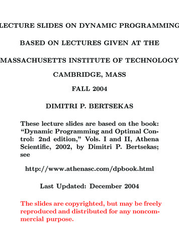
DETERMINISTIC SCHEDULING EXAMPLE Find optimal sequence of operations A, B, C,D (A must precede B and C must precede D)ABC63AB293ACA8Initial56CA2341 0 StateC71ACD3CAB1CAD3CDA2453ACB46CD53 Start from the last tail subproblem and go backwards At each state-time pair, we record the optimalcost-to-go and the optimal decision
STOCHASTIC INVENTORY EXAMPLEwkStock at Period kxkDemand at Period kStock at Period k 1InventorySystemCo s t o f P e rio d kc uk r (xk uk - wk)ukxk 1 xk uk - wkStock Ordered atPeriod k Tail Subproblems of Length 1:JN 1 (xN 1 ) minEuN 1 0 wN 1 cuN 1 r(xN 1 uN 1 wN 1 ) Tail Subproblems of Length N k: Jk (xk ) min E cuk r(xk uk wk )uk 0 wk Jk 1 (xk uk wk )
DP ALGORITHM Start withJN (xN ) gN (xN ),and go backwards using min E gk (xk , uk , wk ) Jk 1 fk (xk , uk , wk ) , k 0, 1, . . . , N 1.Jk (xk ) uk Uk (xk ) wk Then J0 (x0 ), generated at the last step, is equalto the optimal cost J (x0 ). Also, the policyπ {µ 0 , . . . , µ N 1 }where µ k (xk ) minimizes in the right side above foreach xk and k, is optimal. Justification: Proof by induction that Jk (xk )is equal to Jk (xk ), defined as the optimal cost ofthe tail subproblem that starts at time k at statexk . Note that ALL the tail subproblems are solvedin addition to the original problem, and the intensive computational requirements.
PROOF OF THE INDUCTION STEP Let πk µk , µk 1 , . . . , µN 1policy from time k onward denote a tail (x Assume that Jk 1 (xk 1 ) Jk 1k 1 ). Then Jk (xk ) mingk xk , µk (xk ), wkE(µk ,πk 1 ) wk ,.,wN 1 N 1 gN (xN ) min Eµk wkπk 1 min Eµk wk min Eµk wk min gk xk , µk (xk ), wkgi xi , µi (xi ), wi Ewk 1 ,.,wN 1 N 1gN (xN ) gk xk , µk (xk ), wk gi xi , µi (xi ), wii k 1 Jk 1E fk xk , µk (xk ), wkgk xk , µk (xk ), wk Jk 1 fk xk , µk (xk ), wkuk Uk (xk ) wk Jk (xk ) i k 1 min gk (xk , uk , wk ) Jk 1 fk (xk , uk , wk )
LINEAR-QUADRATIC ANALYTICAL EXAMPLEInitialTemperature x0Oven 1Temperatureu0Oven 2Temperatureu1x1FinalTemperature x2 Systemxk 1 (1 a)xk auk ,k 0, 1,where a is given scalar from the interval (0, 1). Costr(x2 T )2 u20 u21where r is given positive scalar. DP Algorithm:J2 (x2 ) r(x2 T )2J1 (x1 ) minu1u21J0 (x0 ) minu0 r (1 a)x1 au1 Tu20 J1 (1 a)x0 au0 2
STATE AUGMENTATION When assumptions of the basic problem areviolated (e.g., disturbances are correlated, cost isnonadditive, etc) reformulate/augment the state. Example: Time lagsxk 1 fk (xk , xk 1 , uk , wk ) Introduce additional state variable yk xk 1 .New system takes the form xk 1yk 1 fk (xk , yk , uk , wk )xk View x̃k (xk , yk ) as the new state. DP algorithm for the reformulated problem: Jk (xk , xk 1 ) minEuk Uk (xk ) wk gk (xk , uk , wk ) Jk 1 fk (xk , xk 1 , uk , wk ), xk
6.231 DYNAMIC PROGRAMMINGLECTURE 3LECTURE OUTLINE Deterministic finite-state DP problems Backward shortest path algorithm Forward shortest path algorithm Shortest path examples Alternative shortest path algorithms
DETERMINISTIC FINITE-STATE PROBLEMTerminal Arcswith Cost Equalto Terminal Cost.tArtificial TerminalNode.Initial States.Stage 0Stage 1Stage 2.Stage N - 1Stage N States ¡ ¿ Nodes Controls ¡ ¿ Arcs Control sequences (open-loop) ¡ ¿ paths frominitial state to terminal states akij : Cost of transition from state i Sk to statej Sk 1 at time k (view it as “length” of the arc) aNit : Terminal cost of state i SN Cost of control sequence ¡ ¿ Cost of the corresponding path (view it as “length” of the path)
BACKWARD AND FORWARD DP ALGORITHMS DP algorithm:JN (i) aNit , i SN ,Jk (i) min akij Jk 1 (j) , i Sk , k 0, . . . , N 1.j Sk 1The optimal cost is J0 (s) and is equal to thelength of the shortest path from s to t. Observation: An optimal path s t is also anoptimal path t s in a “reverse” shortest pathproblem where the direction of each arc is reversedand its length is left unchanged. Forward DP algorithm ( backward DP algorithm for the reverse problem):J N (j) a0sj , j S1 ,J k (j) mini SN k kaN J k 1 (i) , j SN k 1ij The optimal cost is J 0 (t) mini SN aNit J1 (i) . View J k (j) as optimal cost-to-arrive to state jfrom initial state s.
A NOTE ON FORWARD DP ALGORITHMS There is no forward DP algorithm for stochasticproblems. Mathematically, for stochastic problems, wecannot restrict ourselves to open-loop sequences,so the shortest path viewpoint fails. Conceptually, in the presence of uncertainty,the concept of “optimal-cost-to-arrive” at a statexk does not make sense. The reason is that it maybe impossible to guarantee (with prob. 1) that anygiven state can be reached. By contrast, even in stochastic problems, theconcept of “optimal cost-to-go” from any state xkmakes clear sense.
GENERIC SHORTEST PATH PROBLEMS {1, 2, . . . , N, t}: nodes of a graph (t: the destination) aij : cost of moving from node i to node j Find a shortest (minimum cost) path from eachnode i to node t Assumption: All cycles have nonnegative length.Then an optimal path need not take more than Nmoves We formulate the problem as one where we require exactly N moves but allow degenerate movesfrom a node i to itself with cost aii 0.Jk (i) optimal cost of getting from i to t in N k moves.J0 (i): Cost of the optimal path from i to t. DP algorithm:Jk (i) minj 1,.,Naij Jk 1 (j) ,with JN 1 (i) ait , i 1, 2, . . . , N.k 0, 1, . . . , N 2,
EXAMPLEState 5634571513Stage k(b)(a)JN 1 (i) ait ,Jk (i) 4minj 1,.,Ni 1, 2, . . . , N,aij Jk 1 (j) ,k 0, 1, . . . , N 2.
STATE ESTIMATION / HIDDEN MARKOV MODELS Markov chain with transition probabilities pij State transitions are hidden from view For each transition, we get an (independent)observation r(z; i, j): Prob. the observation takes value zwhen the state transition is from i to j Trajectory estimation problem: Given the observation sequence ZN {z1 , z2 , . . . , zN }, what isthe “most likely” state transition sequence X̂N {x̂0 , x̂1 , . . . , x̂N } [one that maximizes p(XN ZN )over all XN {x0 , x1 , . . . , xN }].sx0x1x2xN - 1.xNt
VITERBI ALGORITHM We havep(XNp(XN , ZN ) ZN ) p(ZN )where p(XN , ZN ) and p(ZN ) are the unconditionalprobabilities of occurrence of (XN , ZN ) and ZN Maximizing p(XN ZN ) is equivalent with maximizing ln(p(XN , ZN )) We havep(XN , ZN ) πx0N pxk 1 xk r(zk ; xk 1 , xk )k 1so the problem is equivalent tominimize ln(πx0 ) N ln pxk 1 xk r(zk ; xk 1 , xk )k 1over all possible sequences {x0 , x1 , . . . , xN }. This is a shortest path problem.
GENERAL SHORTEST PATH ALGORITHMS There are many nonDP shortest path algorithms. They can all be used to solve deterministicfinite-state problems They may be preferable than DP if they avoidcalculating the optimal cost-to-go of EVERY state This is essential for problems with HUGE statespaces. Such problems arise for example in combinatorial optimizationA5ABCADAC204ABD3ABCD151AB20Origin Node s4ABDC5Artificial Terminal Node t551 1520 CB5
LABEL CORRECTING METHODS Given: Origin s, destination t, lengths aij 0. Idea is to progressively discover shorter pathsfrom the origin s to every other node i Notation: di (label of i): Length of the shortest pathfound (initially ds 0, di for i s) UPPER: The label dt of the destination OPEN list: Contains nodes that are currently active in the sense that they are candidates for further examination (initially OPEN {s})Label Correcting AlgorithmStep 1 (Node Removal): Remove a node i fromOPEN and for each child j of i, do step 2.Step 2 (Node Insertion Test): If di aij min{dj , UPPER}, set dj di aij and set i tobe the parent of j. In addition, if j t, place j inOPEN if it is not already in OPEN, while if j t,set UPPER to the new value di ait of dt .Step 3 (Termination Test): If OPEN is empty,terminate; else go to step 1.
VISUALIZATION/EXPLANATION Given: Origin s, destination t, lengths aij 0. di (label of i): Length of the shortest pathfound thus far (initially ds 0, di for i s).The label di is implicitly associated with an s ipath. UPPER: The label dt of the destination OPEN list: Contains “active” nodes (initiallyOPEN {s})Is di aij UPPER ?(Does the path s -- i -- jhave a chance to be partof a shorter s -- t path ?)YESSet dj di aijINSERTYESiOPENREMOVEjIs di aij dj ?(Is the path s -- i -- jbetter than thecurrent path s -- j ?)
EXAMPLE1523AOrigin Node s17AB1510AC204203ABC5 ABDACB8 ACD34 ABCD346 ABDCACBD11515AD4ADB4ADC209 ACDB5320ADBC1ADCB5Artificial Terminal Node tIter. No.Node Exiting OPENOPEN after IterationUPPER0-1112, 7,10223, 5, 7, 10334, 5, 7, 10 445, 7, 1043556, 7, 1043667, 1013778, 1013889, 10139910131010Empty13 Note that some nodes never entered OPEN
LABEL CORRECTING METHODS Origin s, destination t, lengths aij that are 0. di (label of i): Length of the shortest pathfound thus far (initially di except ds 0).The label di is implicitly associated with an s ipath. UPPER: Label dt of the destination OPEN list: Contains “active” nodes (initiallyOPEN {s})Is di aij UPPER ?(Does the path s -- i -- jhave a chance to be partof a shorter s -- t path ?)YESSet dj di aijINSERTYESiOPENREMOVEjIs di aij dj ?(Is the path s -- i -- jbetter than thecurrent path s -- j ?)
6.231 DYNAMIC PROGRAMMINGLECTURE 4LECTURE OUTLINE Label correcting methods for shortest paths Variants of label correcting methods Branch-and-bound as a shortest path algorithm
LABEL CORRECTING METHODS Origin s, destination t, lengths aij that are 0. di (label of i): Length of the shortest pathfound thus far (initially di except ds 0).The label di is implicitly associated with an s ipath. UPPER: Label dt of the destination OPEN list: Contains “active” nodes (initiallyOPEN {s})Is di aij UPPER ?(Does the path s -- i -- jhave a chance to be partof a shorter s -- t path ?)YESSet dj di aijINSERTYESiOPENREMOVEjIs di aij dj ?(Is the path s -- i -- jbetter than thecurrent path s -- j ?)
VALIDITY OF LABEL CORRECTING METHODSProposition: If there exists at least one pathfrom the origin to the destination, the label correcting algorithm terminates with UPPER equalto the shortest distance from the origin to the destination.Proof: (1) Each time a node j enters OPEN, itslabel is decreased and becomes equal to the lengthof some path from s to j(2) The number of possible distinct path lengthsis finite, so the number of times a node can enterOPEN is finite, and the algorithm terminates(3) Let (s, j1 , j2 , . . . , jk , t) be a shortest path andlet d be the shortest distance. If UPPER d at termination, UPPER will also be larger thanthe length of all the paths (s, j1 , . . . , jm ), m 1, . . . , k, throughout the algorithm. Hence, nodejk will never enter the OPEN list with djk equalto the shortest distance from s to jk . Similarlynode jk 1 will never enter the OPEN list withdjk 1 equal to the shortest distance from s to jk 1 .Continue to j1 to get a contradiction.
MAKING THE METHOD EFFICIENT Reduce the value of UPPER as quickly as possible Try to discover “good” s t paths early inthe course of the algorithm Keep the number of reentries into OPEN low Try to remove from OPEN nodes with smalllabel first. Heuristic rationale: if di is small, then djwhen set to di aij will be accordingly small,so reentrance of j in the OPEN list is lesslikely. Reduce the overhead for selecting the node tobe removed from OPEN These objectives are often in conflict. They giverise to a large variety of distinct implementations Good practical strategies try to strike a compromise between low overhead and small label nodeselection.
NODE SELECTION METHODS Depth-first search: Remove from the top ofOPEN and insert at the top of OPEN. Has low memory storage properties (OPENis not too long). Reduces UPPER quickly.Origin Node s1210346571189121314Destination Node t Best-first search (Djikstra): Remove fromOPEN a node with minimum value of label. Interesting property: Each node will be inserted in OPEN at most once. Many implementations/approximations
ADVANCED INITIALIZATION Instead of starting from di for all i s,start withdi length of some path from s to i (or di )OPEN {i t di } Motivation: Get a small starting value of UPPER. No node with shortest distance initial valueof UPPER will enter OPEN Good practical idea: Run a heuristic (or use common sense) toget a “good” starting path P from s to t Use as UPPER the length of P , and as dithe path distances of all nodes i along P Very useful also in reoptimization, where wesolve the same problem with slightly different data
VARIANTS OF LABEL CORRECTING METHODS If a lower bound hj of the true shortest distance from j to t is known, use the testdi aij hj UPPERfor entry into OPEN, instead ofdi aij UPPERThe label correcting method with lower bounds asabove is often referred to as the A method. If an upper bound mj of the true shortestdistance from j to t is known, then if dj mj UPPER, reduce UPPER to dj mj . Important use: Branch-and-bound algorithmfor discrete optimization can be viewed as an implementation of this last variant.
BRANCH-AND-BOUND METHOD Problem: Minimize f (x) over a finite set offeasible solutions X. Idea of branch-and-bound: Partition the feasible set into smaller subsets, and then calculatecertain bounds on the attainable cost within someof the subsets to eliminate from further consideration other subsets.Bounding PrincipleGiven two subsets Y1 X and Y2 X, supposethat we have boundsf 1 min f (x),x Y1f 2 min f (x).x Y2Then, if f 2 f 1 , the solutions in Y1 may be disregarded since their cost cannot be smaller thanthe cost of the best solution in Y2 . The B B algorithm can be viewed as a label correcting algorithm, where lower bounds define the arc costs, and upper bounds are used tostrengthen the test for admission to OPEN.
SHORTEST PATH IMPLEMENTATION Acyclic graph/partition of X into subsets (typically a tree). The leafs consist of single solutions. Upper/Lower bounds f Y and f Y for the minimum cost over each subset Y can be calculated. The lower bound of a leaf {x} is f (x) Each arc (Y, Z) has length f Z f Y Shortest distance from X to Y f Y f X Distance from origin X to a leaf {x} is f (x) f X Distance from origin X to a leaf {x} is f (x) f X Shortest path from X to the set of leafs givesthe optimal cost and optimal solution UPPER is the smallest f (x) out of leaf nodes{x} examined so far{1,2,3,4,5}{4,5}{1,2,3}{1,2,}{1}{3}{2}{4}{5}
BRANCH-AND-BOUND ALGORITHMStep 1: Remove a node Y from OPEN. For eachchild Yj of Y , do the following: If f Y j UPPER,then place Yj in OPEN. If in addition f Y j UPPER, then set UPPER f Y j , and if Yj consistsof a single solution, mark that solution as beingthe best solution found so far.Step 2: (Termination Test) If OPEN is nonempty,go to step 1. Otherwise, terminate; the best solution found so far is optimal. It is neither practical nor necessary to generatea priori the acyclic graph (generate it as you go). Keys to branch-and-bound: Generate as sharp as possible upper and lowerbounds at each node Have a good partitioning and node selectionstrategy Method involves a lot of art, may be prohibitivelytime-consuming, but is guaranteed to find an optimal solution.
6.231 DYNAMIC PROGRAMMINGLECTURE 5LECTURE OUTLINE Examples of stochastic DP problems Linear-quadratic problems Inventory control
LINEAR-QUADRATIC PROBLEMS System: xk 1 Ak xk Bk uk wk Quadratic cost Ewkk 0,1,.,N 1x N QN xN N 1 (x k Qk xk u k Rk uk )k 0where Qk 0 and Rk 0 (in the positive (semi)definitesense). wk are independent and zero mean DP algorithm:JN (xN ) x N QN xN , Jk (xk ) min E xk Qk xk u k Rk ukuk Jk 1 (Ak xk Bk uk wk ) Key facts: Jk (xk ) is quadratic Optimal policy {µ 0 , . . . , µ N 1 } is linear:µ k (xk ) Lk xk Similar treatment of a number of variants
DERIVATION By induction verify thatµ k (xk ) Lk xk ,Jk (xk ) x k Kk xk constant,where Lk are matrices given byLk (Bk Kk 1 Bk Rk ) 1 Bk Kk 1 Ak ,and where Kk are symmetric positive semidefinitematrices given byKN QN ,Kk A k Kk 1 Kk 1 Bk (Bk Kk 1 Bk 1 Rk ) Bk Kk 1 Ak Qk . This is called the discrete-time Riccati equation. Just like DP, it starts at the terminal time Nand proceeds backwards. Certainty equivalence holds (optimal policy isthe same as when wk is replaced by its expectedvalue E{wk } 0).
ASYMPTOTIC BEHAVIOR OF RICCATI EQUATION Assume time-independent system and cost perstage, and some technical assumptions: controlability of (A, B) and observability of (A, C) whereQ C C The Riccati equation converges limk Kk K, where K is pos. definite, and is the unique(within the class of pos. semidefinite matrices) solution of the algebraic Riccati equationK A K KB(B KB R) 1 B K A Q The corresponding steady-state controller µ (x) Lx, whereL (B KB R) 1 B KA,is stable in the sense that the matrix (A BL) ofthe closed-loop systemxk 1 (A BL)xk wksatisfies limk (A BL)k 0.
GRAPHICAL PROOF FOR SCALAR SYSTEMS2ARB2 QF(P )Q-R2B P04 50PkPk 1 P*P Riccati equation (with Pk KN k ): Pk 1 A2 Pk B 2 Pk2B 2 Pk R Q,or Pk 1 F (Pk ), whereA2 RP Q.F (P ) 2B P R Note the two steady-state solutions, satisfyingP F (P ), of which only one is positive.
RANDOM SYSTEM MATRICES Suppose that {A0 , B0 }, . . . , {AN 1 , BN 1 } arenot known but rather are independent randommatrices that are also independent of the wk DP algorithm isJN (xN ) x N QN xN ,Jk (xk ) minE uk wk ,Ak ,Bk u k Rk ukx k Qk xk Jk 1 (Ak xk Bk uk wk ) Optimal policy µ k (xk ) Lk xk , where 1 E{Bk Kk 1 Ak },L
LECTURE SLIDES ON DYNAMIC PROGRAMMING BASED ON LECTURES GIVEN AT THE MASSACHUSETTS INSTITUTE OF TECHNOLOGY CAMBRIDGE, MASS FALL 2004 DIMITRI P. BERTSEKAS . Example: Find two-game chess match strategy Timid play draws with prob. p d 0andloses with prob. 1 p d. Bold play wins with prob. p w 1/2 and loses with prob. 1 p w 1 - 0 0 .