Transcription
A Miscellany of Mathematical PhysicsV. Balakrishnan#1
All rights reserved. No parts of this publication may be reproduced, stored in a retrieval system,or transmitted, in any form or by any means, electronic, mechanical, photocopying, recording,or otherwise, without prior permission of the publisher.c Indian Academy of Sciences 2018Reproduced fromResonance – journal of science educationReformatted by :Sriranga Digital Software Technologies Private Limited,Srirangapatna.Printed at:Tholasi Prints India Pvt LtdPublished byIndian Academy of Sciences#2
ForewordThe Masterclass series of eBooks brings together pedagogical articles on single broad topics taken from Resonance, the Journal of Science Education, that has been published monthlyby the Indian Academy of Sciences since January 1996. Primarily directed at students andteachers at the undergraduate level, the journal has brought out a wide spectrum of articles ina range of scientific disciplines. Articles in the journal are written in a style that makes themaccessible to readers from diverse backgrounds, and in addition, they provide a useful sourceof instruction that is not always available in textbooks.The fourth book in the series, ‘A Miscellany of Mathematical Physics’, is by Prof.V. Balakrishnan. A distinguished theoretical physicist, Prof. Balakrishnan worked at TIFR(Mumbai) and RRC (Kalpakkam) before settling down at IIT Madras, from where he retiredas an Emeritus Professor in 2013, after a stint lasting 33 years. Prof. Balakrishnan is widelyrenowned, in India and abroad, as a stimulating and inspiring teacher at all levels, undergraduate to doctoral. He has also contributed pedagogical articles regularly to Resonance, and aselection of these articles, substantially reworked in many cases, comprise the present book.Prof. Balakrishnan is well known for his research contributions to the areas of stochasticprocesses, quantum dynamics, non-linear dynamics and chaos. The book, which will be available in digital format, and will be housed as always on the Academy website, will be valuable toboth students and experts as a useful handbook on diverse topics in theoretical physics, rangingfrom the rotations of vectors and matrices to the many avatars of the Dirac delta function.Amitabh JoshiEditor of PublicationsIndian Academy of SciencesFebruary 2018#3
#4
About the AuthorProf V. Balakrishnan – universally abbreviated to Bala or Balki – needs no introductionto professional physicists of his generation – and indeed many later generations, especiallythose who are theoretically inclined. He also needs no introduction to almost any student whohas passed through the Indian Institute of Technology, Madras in the last thirty years, beingsomething of a legend there. Indeed, many would-be engineers were attracted to physics byhis courses. Thanks to NPTEL and the internet, his lectures have now reached an even largerconstituency, namely engineering and physics students all over the country and ouside. He hasthus been an inspiring figure in the research and teaching community for decades.The target audience of this Masterclass, however, includes young readers who will be encountering him for the first time. The bare facts of his career and achievements have alreadybeen mentioned in the preface, so a more personal note may be appropriate here.I come from roughly one academic generation – five years – after Bala. Long before Iheard him in person, research students of the 1969 batch at the Tata institute of FundamentalResearch in Mumbai wrote to me in faraway Bangalore of how Bala had made a course onspecial functions come alive in the complex plane. I later read his research papers in Pramana,the journal of physics of the Indian Academy of Sciences. Unlike most such papers, these werewritten as if they were meant to be read aloud, combining originality with context, motivation,and lucid exposition. When I eventually met him face to face, our discussions initially centredon statistical physics, but as I soon realized, there was very little in any branch of theoreticalphysics that he had not thought about very deeply.Bala has a first-hand perspective: the mathematics and physics in any discussion with himis served fresh. This is the hallmark of the best teachers, and of people who have thought andworked long and hard and reconstructed their subjects for themselves. These perspectives gowell beyond physics: Bala’s sharp insights into events around him, both academic and nonacademic, have always been a delight to listeners – as much for what is said as for how it isexpressed. All this might leave the reader with a picture of an armchair critical academic but itcould not be more wrong. I was fortunate to see another side of Bala at close quarters, whenserving under his chairmanship on the board of a charitable trust. His handling of difficult,people, situations and decisions was balanced, humane and principled and I am sure this wouldhave characterized his functioning in numerous other roles as well.This collection of articles written originally for Resonance at various points during the pasttwenty or so years (but now considerably revised and enhanced) has been woven into chapters.It takes a deceptively relaxed and informal approach to a formidable subject, and serves as agateway to deeper study. Bala has written and lectured extensively on mathematical methodsused by physicists in various forums, and for a beginning student there is no better place tostart than this Masterclass.Rajaram NityanandaAzim Premji University, Bengaluru#5
#6
PrefaceThis book is based on eight articles that were written for Resonance. Needless to say, thematerial has been rearranged, revised, and considerably expanded in some directions, so as tohave a degree of cogency. The articles themselves grew out of the notion that the mathematicaltools and techniques required by the students of physical sciences can, and should, be introduced to them in a more ‘user-friendly’ style than is generally the case. The initial introductionshould be heuristic, with adequate motivation. The development of the subject matter shouldhelp the student not only to learn the techniques, but also to gain insight and the ability torecognise interconnections. Attention should be paid to the natural unfolding of the subjectmatter; one thing should lead to another. While correctness can never be sacrificed, formalrigour and exactitude need not be at the forefront.In this book, we take a walking tour — or a casual stroll — through a variety of topics,such as vectors, reciprocal vectors, spherical and hyperspherical coordinates, Cartesian tensors,the true meaning of a vector, linear vector spaces, ket and bra vectors, infinitesimal rotationgenerators, the finite rotation formula, rotation matrices, the orthogonal group S O(3) and itsparameter space, Pauli matrices, the unitary group S U(2) and its parameter space, the Diracdelta function, Green functions, the wave equation, its Fourier transform, and its fundamentalsolution in spaces of different dimensions. One thing leads to another!V. Balakrishnan#7
#8
Contents#9What can the answer be?1Oblique axes, reciprocal basis, kets and bras9Reciprocal basis in two dimensions and other nice things15Reciprocal basis in d dimensions and other ramifications21How is a vector rotated?27Rotation matrices and the rotation group35More fun with the rotation group45The many avatars of the Dirac delta function55Signal Propagation: 1. Solution of the Wave Equation67Signal Propagation: 2. Effect of dimensionality75
# 10
What can the answer be? V. BalakrishnanScientific problems are very often first solved by a combination of analogy, educated guesswork and elimination – in short, ‘insight’. The refinements that come later do not make thisearlier process less important. Rather, they generally serve to highlight its value.There is no graded set of lessons by which one progressively gains insight. However, aprofitable line of approach is to ask, at each stage, what the answer to a problem could possibly be, subject to the conditions involved. Techniques such as dimensional analysis, scalingarguments and order-of-magnitude estimates, as well as checks based on limiting values orlimiting cases are part of the armoury in this mode of attack. Elementary vector analysis offersa convenient platform to illustrate this approach.An example from algebraTo set the stage, let us begin with an example in elementary algebra. Consider the determinant1x1x12 (x1 , x2 , x3 ) 1x2x221x3 .x32(1)It is straightforward, of course, to find explicitly by expanding the determinant. But the pointI wish to make here is that can be evaluated almost by inspection, if we note the followingfacts:(i) Multiplying each of x1 , x2 and x3 by some number λ multiplies the value of by λ3 .Thus is a homogeneous function of degree 3.(ii) vanishes if any two of the x’s are equal. Therefore, regarded as a function of x1 , isquadratic with factors (x1 x2 ) and (x1 x3 ); and similarly for x2 and x3 .(iii) changes sign if any two of the x’s are interchanged.Combining these points, we conclude that must be given by (x1 , x2 , x3 ) C(x1 x2 )(x2 x3 )(x3 x1 )where C is some numerical constant. Based on Resonance, Vol. 1, No.8, pp.8-15, 1996.1#1(2)
V. Balakrishnan In order to find the constant C, we have only to look at a simple special case, e.g.,x1 0, x2 1. It is now trivial to simplify the determinant in eq. (1) directly. The resultis (0, 1, x3 ) x3 (x3 1).(3)On the other hand, eq. (2) gives (0, 1, x3 ) Cx3 (x3 1).(4)It follows at once that C must be equal to 1. (Alternatively, match the term x2 x32 obtained bymultiplying together all the diagonal elements of the determinant with the corresponding term C x2 x32 on the right in eq. (2).) Finally, therefore, we have (x1 , x2 , x3 ) (x2 x1 )(x3 x1 )(x3 x2 ).(5)The factors on the right-hand side of eq. (5) have been written in such a way that selecting thefirst term in each bracket yields the product of the diagonal elements of the determinant withthe correct sign.What is important is that our chain of reasoning permits us to generalize this result to thecase of the (n n) determinant (called the Vandermonde determinant)1x1 (x1 , . . . , xn ) .1x2.x1n 1······.x2n 1 · · ·1xn.,(6)xnn 1where n is any integer 2. We can now see that must simply be a product of the n(n 1)/2distinct factors (x j xk ) that can be formed from the variables x1 , . . . , xn . The diagonal element x2 x32 x43 · · · xnn 1 indicates that the sign of each term in is taken care of if we always maintainj k in each factor of (x j xk ). We may therefore deduce the general resultY (x1 , . . . , xn ) (x j xk )(7)1 k j nwithout going through a tedious calculation. This is the spirit in which we shall approach theproblems that follow.Some vector identitiesLet us now go on to vector analysis. As the first example, we consider the derivation of thewell-known identity for the triple cross-product, namely,a (b c) (a · c)b (a · b)c(8)where a, b and c are three arbitrary vectors (in the familiar three-dimensional space). Wewould like to avoid the ‘brute force’ method of writing out components, etc., in some particularcoordinate system. We therefore proceed as follows. Let a (b c) d.2#2
What can the answer be? If a, b and c are three general non-planar vectors in three-dimensional space, any arbitrary vector can be uniquely written as a linear combination of these three vectors.(They serve to define a set of ‘oblique’ axes). But d cannot have any component alonga, because it is a cross product of va with another vector. Therefore, in general, d mustnecessarily be expressible asd βb γc(9)where β and γ are scalars. Note that this argument is valid even in the case of obliqueaxes, i.e., b and c are not required to be perpendicular to a. d is of first order in each of the vectors a, b and c: that is, multiplying any one of themby a constant multiplies the answer by the same constant; further, d vanishes if any ofthese three vectors is zero. Therefore β must be proportional to (a · c) and γ to (a · b),respectively, as these are the only first-order scalars that can be formed from (a, c) and(a, b) respectively. Henced λ(a · c)b µ(a · b)c(10)where λ and µ are absolute constants – dimensionless pure numbers – that are independent of a, b and c. But d changes sign if b and c are interchanged, because c b b c. Therefore d λ(a · b)c µ(a · c)b.(11)Comparison with eq. (10) gives µ λ, so thatd λ[(a · b)c (a · c)b].(12) Having nearly solved the problem, we may now determine λ by looking at an appropriatesimple special case because eq. (12) is valid for all a, b, c. Thus, setting a i, b i, c j (for instance), we get d j by direct evaluation of a (b c), while the right-handside of eq. (12) gives d λ j. Hence λ 1. We thus obtain the general formula quotedin eq. (8).The arguments used above can be repeated to tackle numerous other cases. Let us consider,for instance, the scalar product (a b) · (c d), where a, b, c, d are four arbitrary vectors. Weagain make the following observations: The expression is of first order in each of the four vectors. The presence of the cross products (a b) and (c d) implies that there can be no termsproportional to (a · b) and (c · d) in the result. Hence the answer must be of the form(a b) · (c d) λ(a · c)(b · d) µ(a · d)(b · c)where λ and µ are pure numbers.3#3(13)
V. Balakrishnan As before, since the answer changes sign if a and b are interchanged, we get λ µ. Finally, the overall constant factor is fixed by looking at a special case, e.g., a c i , b d j . This gives λ 1. We thus obtain the familiar formula(a b) · (c d) (a · c)(b · d) (a · d)(b · c).(14)The formulas (8) and (14) are, of course, well known, and several different proofs of theirvalidity can be given. My aim has been to bring out the fact that general considerations oflinearity, symmetry (or antisymmetry), dimensionality, homogeneity, etc. practically determinethe final answer in such problems. This is brought home even more convincingly by the example that follows.Evaluation of an integralWe will first evaluate the surface integralZI4 (a, b, c, d) dΩ (er · a) (er · b) (er · c) (er · d),(15)where the unit vector er varies over the surface of a sphere of unit radius centred at the origin.Here a, b, c, d are four arbitrary constant vectors, which is why I have used the notation I4 .(Such integrals occur in several contexts in physical calculations – for example, in the theory ofcollisions of particles.) A brute force approach to the evaluation of I4 (a, b, c, d) is a formidabletask, but there is a very ‘physical’ way of tackling the problem. We may try to simplify thetask by choosing spherical polar coordinates with the polar axis along one of the given vectors,say a. But this does not help much, because there are three other vectors pointing in arbitrarydirections. Instead, we note that I4 (a, b, c, d) (i) is a scalar, (ii) is of first order in each of thefour vectors a, b, c, d and vanishes if any one of them is zero, and (iii) is totally symmetricunder the interchange of any of these vectors among themselves. Therefore I4 (a, b, c, d) mustnecessarily be of the formI4 (a, b, c, d) λ [(a · b)(c · d) (a · c)(b · d) (a · d)(b · c)] ,(16)where λ is a pure number. The plus signs and the common overall constant λ follow from(iii) above. [I have also used the fact that (a · b)(c · d) (c · d)(a · b), as well as the property(a·b) (b·a).] Likewise, combinations such as (a b)·(c d) are not allowed by this symmetry.(iv) The constant λ is now determined by going over to the special case a b c d k (theunit vector along the polar or z-axis). In that case, since er · k cos θ, the integral reduces bydirect evaluation toZ 1Z 2π4πI4 (k, k, k, k) d(cos θ)dϕ cos4 θ ,(17)5 104#4
What can the answer be?on the one hand; on the other hand, eq. (16) gives I4 (k, k, k, k) 3λ. Hence λ 4π/15,yielding the final answerI4 (a, b, c, d) (4π/15) [(a · b)(c · d) (a · c)(b · d) (a · d)(b · c)] .(18)A generalizationA generalization of the result just derived is tempting and possible! We see at once that allthe odd numbered integrals I1 , I3 , I5 . . . must vanish identically, because there is no way thatwe can form a scalar from an odd number of vectors a, b, c, . . . that satisfies both (ii) and (iii)listed above. What about the corresponding general integral of even order,Z2nY(er · a j ),(19)I2n (a1 , a2 , . . . , a2n ) dΩj 1involving the 2n arbitrary vectors a1 , a2 , . . . , a2n ? The arguments given earlier now lead us toconclude that the value of the integral must be given byX′(20)(a j1 · a j2 ) (a j3 · a j4 ) · · · (a j2n 1 · a j2n ),I2n (a1 , a2 , . . . , a2n ) λpermwhere λ is a constant, yet to be determined, and { j1 , j2 , . . . , j2n } is a permutation of {1, 2, . . . ,2n}. (The prime on the summation sign will be explained shortly.) Now, we know that there are(2n)! permutations of the set {1, 2, . . . , 2n}. However, the number of terms in the summation ineq. (20) is smaller than (2n)!, because of the following restrictions:(i) (a j · ak ) and (ak · a j ) are not to be counted as two distinct quantities.(ii) The order of the n individual factors in a quantity of the form (a j1 ·a j2 ) · · · (a j2n 1 ·a j2n ) doesnot matter. Each such product must appear only once, although there are n! permutationsof the factors in each case.These restrictions bring down the number of terms in the summation in eq. (20) from (2n)! to(2n)!/(2n n!). The prime on the summation sign in eq. (20) is meant to indicate this restrictedsummation.Next, we determine the constant λ by directly evaluating I2n from its defining integral (19)in a simple special case. The most convenient choice is obviously a1 a2 · · · a2n k. Theintegral may then be done by choosing the polar axis to lie along k, so that er · k cos θ.ThereforeZ 14πd(cos θ) (cos θ)2n I2n (k, k, . . . , k) 2π.(21)2n 1 1Equation (20), on the other hand, givesX(2n)! λ′(k · k) n.(22)I2n (k, k, . . . , k) λ2 n!perm5#5
V. BalakrishnanComparing the two expressions, we getλ 2n 2 πn!.(2n 1)!(23)Thus, we arrive at the resultI2n (a1 , a2 , . . . , a2n ) 2n 2 πn! X ′(a j1 · a j2 ) (a j3 · a j4 ) · · · (a j2n 1 · a j2n ).(2n 1)! perm(24)You may check that the result derived earlier, eq. (18), is recovered correctly on setting n 2.A further generalization; hyperspherical coordinatesA further generalization of the result just derived that suggests itself (and which may indeedoccur in actual calculations) is the following. What is the value of the integralZIn,d (a1 , a2 , . . . , an ) dΩ (er · a1 ) . . . (er · an )(25)where er varies over the surface of a unit hypersphere in Euclidean space of d 3 dimensions?The evaluation of this integral gives us an opportunity to introduce and use spherical polarcoordinates in dimensions d 3. These coordinates are called hyperspherical coordinates.It is obvious that, regardless of the value of d, the integral continues to be (i) a scalar, (ii) offirst order in each of the vectors a1 , a2 , . . . , an , and (iii) a totally symmetric function of these nvectors. A moment’s thought then shows that In,d must vanish identically if n is an odd number,for the same reason as before. We are then left with the task of evaluatingI2n,d (a1 , a2 , . . . , a2n ) ZdΩ2nYj 1(er · a j ).(26)As in the case d 3, the answer must necessarily be of the form given by eq. (20), namely,X′(27)(a j1 · a j2 ) (a j3 · a j4 ) · · · (a j2n 1 · a j2n ),I2n,d (a1 , a2 , . . . , a2n ) λpermwhere the summation over the permutations of {1, 2, . . . , 2n} is subject to the same conditionsas before. Once again, it is convenient to determine the value of λ by (i) setting each a j equalto the same unit vector, denoted by k. The result is precisely eq. (22), as before. The argumentPused to compute the number of terms in ′perm is not affected by the dimensionality of the spaceconcerned.We must now evaluate the integralZI2n,d (k, k, . . . , k) dΩ (er · k)2n(28)6#6
What can the answer be?over the surface of a hypersphere of unit radius in d-dimensions. For this purpose we mustspecify hyperspherical coordinates in d dimensions, generalizing the familiar spherical polarcoordinates of 3-dimensional space. Let x1 , x2 , . . . , xd be the Cartesian coordinates of any pointwith position vector r in the space. The hyperspherical coordinates of r are given byr (r, θ1 , θ2 , . . . θd 2 , ϕ),(29)where r is the radial distance of the point from the origin of coordinates. The ranges of thehyperspherical coordinates are0 r , 0 θk π (1 k d 2), 0 ϕ 2π.(30)That is, there are d 2 ‘polar’ angles θk and a single ‘azimuthal’ angle ϕ. These coordinatesare related to the Cartesian coordinates of r according tox1x2x3···xd 1xd r cos θ1r sin θ1 cos θ2r sin θ1 sin θ2 cos �r sin θ1 sin θ2 . . . sin θd 2 cos ϕr sin θ1 sin θ2 . . . sin θd 2 sin ϕ.The solid angle element dΩ can be shown to be dΩ (sin θ1 )d 2 (sin θ2 )d 3 · · · (sin θd 2 ) dθ1 dθ2 · · · dθd 2 dϕ.(31)(32)The next step is to choose k in the most convenient manner. Clearly, it is simplest to chooseit to be the unit vector along the x1 -direction. (This is the analogue of choosing the polar orz-axis along k in the 3-dimensional case.) Then (er · k) is just cos θ1 . Equation (28) givesZ πI2n,d (k, k, . . . , k) 2πdθ1 (sin θ1 )d 2 (cos θ1 )2n0 d 2 ZYπdθk (sin θk )d k 1 .(33)0k 2The definite integrals involved are standard integrals whose values are tabulated. (I shall notdigress into the derivation of those results here.) Using these known values and simplifyingthe expressions obtained in eq. (22) enables us to determine λ. Inserting the result in eq. (27),we arrive at the answer for λ. It is most compactly expressed in terms of the so-called gammafunction, and is given byπd/2 . (34)λ 2n 1 Γ n 12 d7#7
V. BalakrishnanIn simpler terms, this formula reduces to the following: for even values of d, we haveλ For odd values of d,λ πd/2 . 2n 1 n 21 d 1 ! π(d 1)/2 2n d n 21 (d 1) !(2n d 1)!(35).Insertion of these expressions in eq. (27) completes the solution.8#8(36)
Oblique axes, reciprocal basis, kets and bras V. BalakrishnanIn this chapter, we shall see how concepts such as reciprocal basis vectors, dual spaces andco-vectors can be motivated from simple considerations starting from well-known identities inelementary vector analysis.Resolution of a vector along oblique axesLet us begin with the resolution of an ordinary vector v in three-dimensional (Euclidean) space,according tov i v x j vy k vz .(1)What are v x , vy and vz in terms of v? Clearly, v x i · v, vy j · v, and vz k · v. Therefore,if we introduce the projection operator P x ii (note that there is no dot or cross in betweenthe two vectors !), and ‘operate’ with it on the arbitrary vector v by taking the dot product, theresult is precisely ii · v i(i · v) iv x , the component or part of v that lies along the unit vectori. Similarly, we have projection operators Py jj and Pz kk. The unit operator (the operatorthat leaves any vector v unchanged) is clearly just the sum of all the projection operators, namely,I P x Py Pz ii jj kk.(2)This is called the resolution of the identity operator. Thus eq. (1) expresses the fact thatv I v i(i · v) j(j · v) k(k · v).(3)We now ask: what is the counterpart of eq. (3) in the case of oblique axes defined by threearbitrary, non-coplanar vectors a, b and c, instead of the rectangular axes defined by i, j and k?Once again, we can arrive at the answer by figuring out what the answer can possibly be.Writingv α a β b γ c,(4)we observe that the coefficient α cannot involve any overlap‡ of v with either b or c; β cannotinvolve any overlap of v with either c or a; and γ cannot involve any overlap of v with either a orb. This assertion is more or less obvious when the vectors a, b and c are mutually perpendicular.As we are dealing here with oblique axes, however, some elaboration is required. Suppose we Based on Resonance, Vol. 1, No.10, pp. 6-13, 1996.You are familiar with the dot product a · b (also called the scalar product) of two vectors a and b, as well as thecross product a b (also called the vector product) of the two vectors. The object ab is called the tensor product ofthe two vectors. In the present context, it is an operator that acts on a vector to produce another vector.‡‘Overlap’ here refers to the dot or scalar product (also called the inner product) of the vectors concerned. 9#9
V. Balakrishnankeep α fixed at some value, and let β and γ vary. The varying part of v then is then restrictedto a plane parallel to the plane formed by the vectors b and c. All vectors in this plane havethe same value of α, but their projections on the plane formed by b and c vary. Hence α cannotdepend on that projection for any given v. It can only depend on the projection of v onto avector normal to the plane formed by b and c, i.e, onto the vector b c. Therefore α must be proportional to (b c) · v . Similar conclusions hold good for the coefficients β and γ. Hence v λ a (b c) · v µ b (c a) · v ν c (a b) · v ,(5)where the scalar factors λ, µ and ν are yet to be determined. The equivalence of all directionsin space (“the isotropy of space”) implies that λ, µ and ν must be equal to each other. Setting v a, b and c in turn, we find immediately that λ µ ν 1/ (a b) · c .§ Therefore a (b c) · v b (c a) · v c (a b) · vv .(6) (a b) · cBefore discussing the properties of this expansion, let us consider another, equally instructive, way to arrive at it. We begin with the well-known vector identityu (b c) b (u · c) c (u · b).(7)(Recall that a proof of eq. (7) based on general arguments was given in ch. 1.) Now suppose uitself is of the form u v a . Substitution in eq. (7) gives (v a) (b c) b (v a) · c c (v a) · b .(8)The vector representing the quadruple cross product on the left-hand side is thus a linear combination of the vectors b and c. It therefore lies in the plane formed by these two vectors.However, we could as well have written b c d, in which case(v a) (b c) (v a) d a (v · d) v (a · d) a v · (b c) v a · (b c) .(9)The same vector is therefore a linear combination of the two vectors a and v, and thus lies inthe plane formed by them. As the four vectors v, a, b and c may be chosen quite arbitrarily,this appears to be paradoxical. However, we must now recall that these are vectors in threedimensional space, in which no more than three vectors of a given set of vectors can be linearlyindependent, i.e., non-coplanar. In other words, if the vectors a, b and c are a linearly independent set, the fourth vector v must be expressible as a linear combination of these, precisely byequating the expressions found in eqs (8) and (9) and solving for v. The result, after using onceagain the cyclic symmetry of the scalar triple product and some rearrangement, is preciselyeq. (6). This is the counterpart of the resolution in eq. (3) of an arbitrary vector v in a basis oforthogonal axes.§Here we have used the cyclic symmetry of the scalar triple product, namely, (a b) · c (b c) · a (c a) · b.10# 10
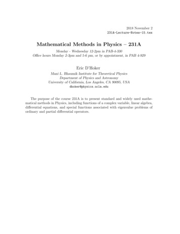
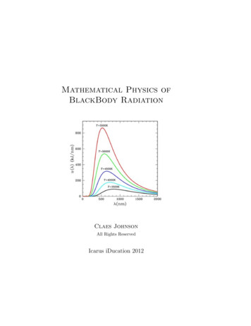
Oblique axes, reciprocal basis, kets and brascbaFigure 1: The volume of the parallelepiped formed by the vectors (a, b, c) is the magnitude oftheir scalar triple product.The reciprocal basisThe answer to the problem of resolving a vector v in an arbitrary basis {a, b, c} is thusv a(A · v) b(B · v) c(C · v),whereA b cc aa b, B , C ,VVV(10)(11)and V (a b) · c. The symbol V has been used because V is the volume of the parallelepipedformed by the vectors a, b and c (see Figure 1). The set of vectors {A, B, C} forms the socalled reciprocal basis. The terminology is most familiar in crystallography: if a, b, c are theprimitive basis vectors of a lattice, then A, B, C are the basis vectors of the ‘reciprocal’ lattice.It is immediately verified thatA · a B · b C · c 1,(12)which helps explain why the term ‘reciprocal basis’ is used. Further,A·b A·c B·a B·c C·a C·b 0.(13)In fact, the reciprocal basis is defined in books on crystallography by eqs (12) and (13): theycan be solved for A, B and C, to obtain precisely the expressions in eq. (11). It is easy to checkthat the general formula of eq. (10) reduces to eq. (3) in the special case of an orthogonal basis.In what space does the reciprocal basis (A, B, C) ‘live’? If the original basis vectors a, band c have the physical dimensions of length, eqs (11) show immediately that A, B and C havethe physical dimensions of (length) 1 . In crystallography and lattice dynamics this fact is usedto define a ‘reciprocal lattice’ in wavenumber space, in which (A, B, C) are the primitive latticevectors. Why does one do this ? It is not my intention to go into lattice dynamics or crystalphysics here, but two good reasons (among several others) may be cited.11# 11
V. Balakrishnan(i) In crystal physics, we have very frequently to deal with periodic functions, i.e., functionsthat satisfy f (er ) f (er R) where R is any lattice vector. That is,R ma nb pc,(14)where m, n and p take on integer values. Such a function can be expanded in a Fourier seriesof the formX(15)fG ei G·er .f (er ) GHere, the sum over G runs over the vectors of the reciprocal lattice, i.e.,G hA kB lC,(16)where (h , k , l) are integers.(ii) The second noteworthy point is that the Bragg condition for diffraction (of X-rays, electrons, neutrons, etc.) from a crystal is expressible in a very simp
The fourth book in the series, 'A Miscellany of Mathematical Physics', is by Prof. V. Balakrishnan. A distinguished theoretical physicist, Prof. Balakrishnan worked at TIFR (Mumbai) and RRC (Kalpakkam) before settling down at IIT Madras, from where he retired as an Emeritus Professor in 2013, after a stint lasting 33 years. Prof.